一种强耦合预估-校正浸入边界法

张和涛; 宁建国; 许香照; 马天宝

doi:10.11883/bzycj-2021-0129

一种强耦合预估-校正浸入边界法

doi: 10.11883/bzycj-2021-0129

北京理工大学爆炸科学与技术国家重点实验室，北京 100081

基金项目: 国家自然科学基金（12032006, 11772061）

详细信息

作者简介:
张和涛（1992－　），男，博士，7520210150@bit.edu.cn

通讯作者:
马天宝（1981－　），男，博士，教授，madabal@bit.edu.cn

中图分类号: O354; O357
计量
- 文章访问数: 646
- HTML全文浏览量: 272
- PDF下载量: 82
- 被引次数: 2
出版历程
- 收稿日期: 2021-04-14
- 修回日期: 2021-05-06
- 网络出版日期: 2021-08-09
- 刊出日期: 2021-09-14

A strong coupling prediction-correction immersed boundary method

State Key Laboratory of Explosion Science and Technology, Beijing Institute of Technology, Beijing 100081, China

摘要

摘要: 为克服传统浸入边界法的质量不守恒缺陷，提出了一种用于可压缩流固耦合问题的强耦合预估-校正浸入边界法。通过阐述一般流固耦合系统的矩阵表示，推导了流固耦合系统的强耦合Gauss-Seidel迭代格式，进一步导出预估-校正格式，提出了预估-校正浸入边界法。该方法使用无耦合边界模型对流体进行预估，将流固耦合边界视为自由面，固体原本占据的空间初始化为零质量的单元，允许流体自由穿过耦合边界。对于流体的计算，使用带有minmod限制器的二阶MUSCL有限体积格式和基于Zha-Bilgen分裂的AUSM⁺-up方法，配合三阶Runge-Kutta格式推进时间步。在校正步骤中，通过一组质量守恒的输运规则来实现输运过程。输运算法可概括为将边界内侧的流体进行标记，根据标记顺序以均匀方式分割和移动流体，产生一个指向边界外侧的流动，最后在边界附近施加速度校正保证无滑移条件。标记和输运算法避免了繁琐的对截断单元的几何处理，确保了算法易于实现。对于固体的计算，分别采用一阶差分格式和隐式动力学有限元格式求解刚体和线弹性体，并利用高斯积分获得固体表面的耦合力。使用预估-校正浸入边界法计算了一维问题和二维问题。在一维活塞问题中，获得了压力分布、相对质量历史和误差曲线，并与其他方法进行了对比。在二维的激波冲击平板问题中，获得了数值模拟纹影和平板结构的挠度历史，并与实验结果进行了对比。研究表明，该方法区别于传统的虚拟网格方法和截断单元方法，能够精确地维持流场的质量守恒并易于实现，且具有一阶收敛精度，能够较准确地预测激波绕射后的流场以及平板在激波作用下的挠度，为开发流固耦合算法提供了一种新的思路。
- 浸入边界法 /
- 流固耦合 /
- 预估-校正 /
- 强耦合 /
- 可压缩流体
Abstract: In the traditional immersed boundary methods for solving compressible fluid-structure interaction problems, conservation is one of the problems that must be considered. When the coupling boundary moves on the fixed grid, the structure coverage will change, resulting in many dead elements and emerging elements on the fluid grid. In the ghost-cell immersed boundary method, the reconstructed grid can not maintain the strict mass conservation when the dead elements and emerging elements appear. In order to overcome the shortcomings of traditional methods, a strong coupling prediction-correction immersed boundary method for compressible fluid-structure interaction problems was proposed. Firstly, the matrix representation of a general fluid-structure coupling system was described, and a strong coupling Gauss-Seidel iterative scheme of fluid-structure coupling system was derived. Furthermore, a prediction-correction scheme was derived, and a prediction-correction immersed boundary method was proposed. The fluid-structure coupling boundary was regarded as a free surface, and the space originally occupied by the solid was initialized as zero mass elements, allowing the fluid to pass through the coupling boundary freely. For the calculation of fluid, the second-order MUSCL finite volume scheme with the minmod limiter and the AUSM⁺-up flux based on Zha-Bilgen splitting were used to advance the time step with the third-order Runge-Kutta scheme. In the correction step, the transport process was realized by a set of mass conservation transport rules. The transport algorithm could be summarized as marking the fluid inside the boundary, dividing and moving the fluid in a uniform way according to the marking order, generating a flow pointing to the outside of the boundary, and finally applying a velocity correction near the boundary to ensure the no-slip condition. The marking and transport algorithm avoided the tedious geometric treatment of the cut-cells, and ensured the easy implementation of the algorithm. For the calculation of solids, the first-order difference scheme and the implicit dynamic finite element scheme were used to solve the rigid body and linear elastic body respectively, and the Gauss quadrature was used to obtain the coupling force on the solid surface. The one-dimensional and two-dimensional problems were calculated by the prediction-correction immersed boundary method. In the one-dimensional piston problem, the accuracy, conservation and convergence of the method were investigated by comparing the results with those in the literature. In the two-dimensional shock wave impact problem, the experimental optical schlieren images were compared with those obtained by the numerical simulation, and the deflection history of the plate structure was investigated. The study shows that this method can accurately maintain the mass conservation of the flow field and has the advantage of easy implementation, which is different from the traditional ghost-cell method and the cut-cell method. This method has the first-order convergence accuracy, and can accurately predict the flow field after shock diffraction and the deflection of plate under shock waves. It provides a new idea for the development of fluid-structure coupling algorithms.
- immersed boundary method /
- fluid-structure interaction /
- prediction-correction /
- strong coupling /
- compressible fluid

HTML全文

辐射流体力学在武器物理、惯性约束聚变、磁约束聚变、地质学和天体物理等诸多领域有广泛的应用，描述多物理过程耦合的辐射流体力学方程组具有强耦合、强间断、强非线性等特征，很难得到解析解，利用计算机进行数值求解是重要的研究手段。

数值模拟是否正确求解了方程，模拟结果能否再现真实的物理过程，都需要对数值模拟程序进行验证与确认^[1-3]。人为构造解方法^[4]是程序验证的重要方法之一，对某些特殊需求(正确性验证、收敛性考察，等)具有不可替代性。在求解双曲型流体力学方程组程序人为解验证方面已有很好的工作^[5-14]，但大多基于欧氏方程，对抛物型辐射扩散方程解析解及人为解验证方面也有很多工作^[15-16]，而适用于求解辐射与流体耦合方程组及拉氏程序验证的人为解模型尚不多见。

针对拉氏辐射流体力学程序正确性验证的需要，文献[17-18]中构造了一类一维拉氏流体力学和辐射流体力学人为解模型，但一维模型的网格运动仅改变网格点的疏密，不涉及到网格的变形，而网格随流体运动而变形是拉氏计算的特点，因此，构造适应流体大变形的二维拉氏辐射流体力学人为解模型对实际应用程序的正确性验证很有意义。本文中基于二维坐标变换关系式，研究了拉氏辐射流体力学人为解方法，构造了适用于辐射流体力学程序验证的二维人为解模型，并应用于非结构拉氏应用程序LAD2D^[19]辐射流体力学计算的正确性考核，取得了很好的效果。

1. 二维拉氏辐射流体力学方程组

考虑如下拉氏形式的二维辐射流体力学方程组：

$\frac{{{\rm{d}}\rho }}{{{\rm{d}}t}} = - \rho \left( {\frac{{\partial u}}{{\partial x}} + \frac{{\partial v}}{{\partial y}}} \right)$

(1)

$\frac{{{\rm{d}}u}}{{{\rm{d}}t}} = - \frac{1}{\rho }\frac{{\partial p}}{{\partial x}} + {s_u}$

(2)

$\frac{{{\rm{d}}v}}{{{\rm{d}}t}} = - \frac{1}{\rho }\frac{{\partial p}}{{\partial y}} + {s_v}$

(3)

$\frac{{{\rm{d}}e}}{{{\rm{d}}t}} = - \frac{p}{\rho }\left( {\frac{{\partial u}}{{\partial x}} + \frac{{\partial v}}{{\partial y}}} \right) + \frac{1}{\rho }\nabla \cdot \left( {\kappa \nabla T} \right) + {s_e}$

(4)

式中： $\frac{\text{d}}{\text{d}t}=\frac{\partial }{\partial t}+u\frac{\partial }{\partial x}+v\frac{\partial }{\partial y}$ 为拉氏随体导数，(x, y, t)为欧氏时空坐标，ρ为密度，u、v分别为x、y方向的流体速度，s_u、s_v为动量方程源项，s_e为能量方程源项，e为比内能，p为压力，T为温度，κ为导热系数。给定状态方程：

$\begin{array}{*{20}{c}} {p = p\left( {\rho ,T} \right),}&{e = e\left( {\rho ,T} \right),}&{\kappa = \kappa \left( {\rho ,T} \right)} \end{array}$

(5)

和适当的初边值条件，则计算模型封闭。

2. 二维拉氏辐射流体力学人为解构造

2.1 二维坐标变换

引入拉氏坐标x₀=(x₀, y₀), 给定拉氏空间(x₀, y₀, τ)到欧氏空间(x, y, t)的坐标变换关系式：

$x = x\left( {{x_0},{y_0},\tau } \right),\;\;\;\;y = y\left( {{x_0},{y_0},\tau } \right),t = \tau$

(6)

其微分关系为：

${\rm{d}}x = \frac{{\partial x}}{{\partial {x_0}}}{\rm{d}}{x_0} + \frac{{\partial x}}{{\partial {y_0}}}{\rm{d}}{y_0} + \frac{{\partial x}}{{\partial \tau }}{\rm{d}}\tau ,\\{\rm{d}}y = \frac{{\partial y}}{{\partial {x_0}}}{\rm{d}}{x_0} + \frac{{\partial y}}{{\partial {y_0}}}{\rm{d}}{y_0} + \frac{{\partial y}}{{\partial \tau }}{\rm{d}}\tau ,\;\;\;\;\;{\rm{d}}t = {\rm{d}}\tau$

(7)

记J(x₀, y₀, τ)为坐标变换的Jacobi矩阵：

$\mathit{\boldsymbol{J}}\left( {{x_0},{y_0},\tau } \right) = \left( {\begin{array}{*{20}{c}} {{J_{11}}}&{{J_{12}}}\\ {{J_{21}}}&{{J_{22}}} \end{array}} \right) = \left( {\begin{array}{*{20}{c}} {\frac{{\partial x\left( {{x_0},{y_0},\tau } \right)}}{{\partial {x_0}}}}&{\frac{{\partial x\left( {{x_0},{y_0},\tau } \right)}}{{\partial {y_0}}}}\\ {\frac{{\partial y\left( {{x_0},{y_0},\tau } \right)}}{{\partial {x_0}}}}&{\frac{{\partial y\left( {{x_0},{y_0},\tau } \right)}}{{\partial {y_0}}}} \end{array}} \right)$

(8)

其行列式记为：

$J = \left| {\begin{array}{*{20}{c}} {\frac{{\partial x}}{{\partial {x_0}}}}&{\frac{{\partial x}}{{\partial {y_0}}}}\\ {\frac{{\partial y}}{{\partial {x_0}}}}&{\frac{{\partial y}}{{\partial {y_0}}}} \end{array}} \right| = \frac{{\partial x}}{{\partial {x_0}}}\frac{{\partial y}}{{\partial {y_0}}} - \frac{{\partial x}}{{\partial {y_0}}}\frac{{\partial y}}{{\partial {x_0}}}$

(9)

$\begin{array}{*{20}{c}} {u\left( {{x_0},{y_0},\tau } \right) = \frac{{\partial x\left( {{x_0},{y_0},\tau } \right)}}{{\partial \tau }},}&{v\left( {{x_0},{y_0},\tau } \right) = \frac{{\partial y\left( {{x_0},{y_0},\tau } \right)}}{{\partial \tau }}} \end{array}$

(10)

为流体速度。

函数u(x₀, y₀, τ)、v(x₀, y₀, τ)与坐标变换的Jacobi矩阵J(x₀, y₀, τ)应满足Cauchy相容关系：

$\begin{array}{*{20}{c}} {\frac{{\partial u}}{{\partial {x_0}}} = \frac{{\partial {J_{11}}}}{{\partial \tau }},}&{\frac{{\partial u}}{{\partial {y_0}}} = \frac{{\partial {J_{12}}}}{{\partial \tau }};}&{\frac{{\partial v}}{{\partial {x_0}}} = \frac{{\partial {J_{21}}}}{{\partial \tau }},}&{\frac{{\partial v}}{{\partial {y_0}}} = \frac{{\partial {J_{22}}}}{{\partial \tau }}} \end{array}$

(11)

下面给出欧氏空间中的空间导数和拉氏随体导数在拉氏空间的表达式。

设物理变量z在欧氏空间关于坐标(x, y, t)的函数关系为f，在拉氏空间关于坐标(x₀, y₀, τ)的函数关系为g，即：

$\begin{array}{*{20}{c}} {z = f\left( {x,y,t} \right) = f\left[ {x\left( {{x_0},{y_0},\tau } \right),y\left( {{x_0},{y_0},\tau } \right),\tau } \right] \equiv }\\ {g\left( {{x_0},{y_0},\tau } \right) = g\left[ {x\left( {{x_0},{y_0},\tau } \right),y\left( {{x_0},{y_0},\tau } \right),t} \right] \equiv f\left( {x,y,t} \right)} \end{array}$

(12)

则有：

$\begin{array}{*{20}{c}} {\frac{{\partial z}}{{\partial {x_0}}} = \frac{{\partial g\left( {{x_0},{y_0},\tau } \right)}}{{\partial {x_0}}} = \frac{{\partial f\left[ {x\left( {{x_0},{y_0},\tau } \right),y\left( {{x_0},{y_0},\tau } \right),\tau } \right]}}{{\partial {x_0}}} = }\\ {\frac{{\partial f\left( {x,y,t} \right)}}{{\partial x}}\frac{{\partial x\left( {{x_0},{y_0},\tau } \right)}}{{\partial {x_0}}} + \frac{{\partial f\left( {x,y,t} \right)}}{{\partial y}}\frac{{\partial y\left( {{x_0},{y_0},\tau } \right)}}{{\partial {x_0}}} = \frac{{\partial z}}{{\partial x}}\frac{{\partial x}}{{\partial {x_0}}} + \frac{{\partial z}}{{\partial y}}\frac{{\partial y}}{{\partial {x_0}}}} \end{array}$

(13)

$\begin{array}{*{20}{c}} {\frac{{\partial z}}{{\partial {y_0}}} = \frac{{\partial g\left( {{x_0},{y_0},\tau } \right)}}{{\partial {y_0}}} = \frac{{\partial f\left[ {x\left( {{x_0},{y_0},\tau } \right),y\left( {{x_0},{y_0},\tau } \right),\tau } \right]}}{{\partial {y_0}}} = }\\ {\frac{{\partial f\left( {x,y,t} \right)}}{{\partial x}}\frac{{\partial x\left( {{x_0},{y_0},\tau } \right)}}{{\partial {y_0}}} + \frac{{\partial f\left( {x,y,t} \right)}}{{\partial y}}\frac{{\partial y\left( {{x_0},{y_0},\tau } \right)}}{{\partial {y_0}}} = \frac{{\partial z}}{{\partial x}}\frac{{\partial x}}{{\partial {y_0}}} + \frac{{\partial z}}{{\partial y}}\frac{{\partial y}}{{\partial {y_0}}}} \end{array}$

(14)

假定坐标变换Jacobi行列式 $J=\frac{\partial x}{\partial {{x}_{0}}}\frac{\partial y}{\partial {{y}_{0}}}-\frac{\partial x}{\partial {{y}_{0}}}\frac{\partial y}{\partial {{x}_{0}}}\ne 0$ ，由式(13)~(14)可以解出欧氏空间导数：

$\begin{array}{*{20}{c}} {\frac{{\partial z}}{{\partial x}} = \frac{1}{J}\left( {\frac{{\partial z}}{{\partial {x_0}}}\frac{{\partial y}}{{\partial {y_0}}} - \frac{{\partial z}}{{\partial {y_0}}}\frac{{\partial y}}{{\partial {x_0}}}} \right),}&{\frac{{\partial z}}{{\partial y}} = \frac{1}{J}\left( {\frac{{\partial z}}{{\partial {y_0}}}\frac{{\partial x}}{{\partial {x_0}}} - \frac{{\partial z}}{{\partial {x_0}}}\frac{{\partial x}}{{\partial {y_0}}}} \right)} \end{array}$

(15)

而:

$\begin{array}{*{20}{c}} {\frac{{\partial z}}{{\partial \tau }} = \frac{{\partial g\left( {{x_0},{y_0},\tau } \right)}}{{\partial \tau }} = \frac{{\partial f\left[ {x\left( {{x_0},{y_0},\tau } \right),y\left( {{x_0},{y_0},\tau } \right),\tau } \right]}}{{\partial \tau }} = }\\ {\frac{{\partial f\left( {x,y,t} \right)}}{{\partial t}}\frac{{\partial f\left( {x,y,t} \right)}}{{\partial x}} + \frac{{\partial x\left( {{x_0},{y_0},\tau } \right)}}{{\partial \tau }} + \frac{{\partial f\left( {x,y,t} \right)}}{{\partial y}}\frac{{\partial y\left( {{x_0},{y_0},\tau } \right)}}{{\partial \tau }} = \frac{{{\rm{d}}f}}{{{\rm{d}}t}} = \frac{{{\rm{d}}z}}{{{\rm{d}}t}}} \end{array}$

即欧氏空间的拉氏随体导数就等于拉氏空间的时间导数：

$\frac{{{\rm{d}}z\left( {x,y,t} \right)}}{{{\rm{d}}t}} = \frac{{\partial z\left( {{x_0},{y_0},\tau } \right)}}{{\partial \tau }}$

(16)

2.2 二维拉氏辐射流体力学人为解构造方法

从拉氏计算中使用的二维拉氏辐射流体力学方程(1)~(5)出发，给定位移解函数和温度解函数，利用二维坐标变换关系式，由无源项的质量方程解出密度解函数，再将已知解函数代入动量方程和能量方程，残余项视为方程源项。具体构造过程如下:

(1) 给定位移解函数x=x(x₀, y₀, τ)，y=y(x₀, y₀, τ)和温度解函数T=T(x₀, y₀, τ)。

(2) 根据式(9)和(10)，由位移解函数x=x(x₀, y₀, τ), y=y(x₀, y₀, τ), 可计算出坐标变换Jacobi行列式J=J(x₀, y₀, τ)和流体速度u=u(x₀, y₀, τ), v=v(x₀, y₀, τ)。

(3) 解连续性方程求出密度解函数。

利用空间导数关系式(15)和Cauchy相容关系式(11)求出速度散度：

$\begin{array}{*{20}{c}} {\nabla \cdot \mathit{\boldsymbol{v}} = \frac{{\partial u}}{{\partial x}} + \frac{{\partial v}}{{\partial y}} = \frac{1}{J}\left( {\frac{{\partial u}}{{\partial {x_0}}}\frac{{\partial y}}{{\partial {y_0}}} - \frac{{\partial u}}{{\partial {y_0}}}\frac{{\partial y}}{{\partial {x_0}}}} \right) + \frac{1}{J}\left( {\frac{{\partial v}}{{\partial {y_0}}}\frac{{\partial x}}{{\partial {x_0}}} - \frac{{\partial v}}{{\partial {x_0}}}\frac{{\partial x}}{{\partial {y_0}}}} \right) = }\\ {\frac{1}{J}\left[ {\frac{\partial }{{\partial \tau }}\left( {\frac{{\partial x}}{{\partial {x_0}}}} \right)\frac{{\partial y}}{{\partial {y_0}}} - \frac{\partial }{{\partial \tau }}\left( {\frac{{\partial x}}{{\partial {y_0}}}} \right)\frac{{\partial y}}{{\partial {x_0}}}} \right] + \frac{1}{J}\left[ {\frac{\partial }{{\partial \tau }}\left( {\frac{{\partial y}}{{\partial {y_0}}}} \right)\frac{{\partial x}}{{\partial {x_0}}} - \frac{\partial }{{\partial \tau }}\left( {\frac{{\partial y}}{{\partial {x_0}}}} \right)\frac{{\partial x}}{{\partial {y_0}}}} \right] = }\\ {\frac{1}{J}\left[ {\frac{\partial }{{\partial \tau }}\left( {\frac{{\partial x}}{{\partial {x_0}}}} \right)\frac{{\partial y}}{{\partial {y_0}}} + \frac{\partial }{{\partial \tau }}\left( {\frac{{\partial y}}{{\partial {y_0}}}} \right)\frac{{\partial x}}{{\partial {x_0}}} - \frac{\partial }{{\partial \tau }}\left( {\frac{{\partial x}}{{\partial {y_0}}}} \right)\frac{{\partial y}}{{\partial {x_0}}} - \frac{\partial }{{\partial \tau }}\left( {\frac{{\partial y}}{{\partial {x_0}}}} \right)\frac{{\partial x}}{{\partial {y_0}}}} \right] = }\\ {\frac{1}{J}\left[ {\frac{\partial }{{\partial \tau }}\left( {\frac{{\partial x}}{{\partial {x_0}}}\frac{{\partial y}}{{\partial {y_0}}} - \frac{{\partial x}}{{\partial {y_0}}}\frac{{\partial y}}{{\partial {x_0}}}} \right)} \right] = \frac{1}{J}\frac{{\partial J}}{{\partial \tau }}} \end{array}$

(17)

代入连续性方程(1)，并利用欧氏空间的拉氏随体导数与拉氏空间的时间导数之间的关系式(16)，得：

$\frac{{\partial \rho \left( {{x_0},{y_0},\tau } \right)}}{{\partial \tau }} = - \rho \left( {{x_0},{y_0},\tau } \right)\frac{1}{{J\left( {{x_0},{y_0},\tau } \right)}}\frac{{\partial J\left( {{x_0},{y_0},\tau } \right)}}{{\partial \tau }}$

即 $J\frac{\partial \rho }{\partial \tau }+\rho \frac{\partial J}{\partial \tau }=0$ ，进一步改写为 $\frac{\partial \left(\rho J \right)}{\partial \tau }=0$ ，可得出密度解函数的精确表达式：

$\rho \left( {{x_0},{y_0},\tau } \right) = \frac{{{\rho _0}\left( {{x_0},{y_0}} \right){J_0}\left( {{x_0},{y_0}} \right)}}{{J\left( {{x_0},{y_0},\tau } \right)}}$

(18)

式中：ρ₀(x₀, y₀)=ρ(x₀, y₀, 0)，J₀(x₀, y₀)=J(x₀, y₀, 0)。

(4) 根据温度解函数确定动量方程源项和内能方程源项。

由动量方程(2)~(3)导出源项：

$\begin{array}{*{20}{c}} {{s_u} = \frac{{{\rm{d}}u}}{{{\rm{d}}t}} + \frac{1}{\rho }\frac{{\partial p}}{{\partial x}},}&{{s_v} = \frac{{{\rm{d}}v}}{{{\rm{d}}t}} + \frac{1}{\rho }\frac{{\partial p}}{{\partial y}}} \end{array}$

(19)

根据时间导数关系式(16)和空间导数关系式(15)，可得：

$\begin{array}{*{20}{c}} {{s_u} = \frac{{\partial u\left( {{x_0},{y_0},\tau } \right)}}{{\partial \tau }} + \frac{1}{{\rho \left( {{x_0},{y_0},\tau } \right)J\left( {{x_0},{y_0},\tau } \right)}} \cdot }\\ {\left[ {\frac{{\partial p\left( {{x_0},{y_0},\tau } \right)}}{{\partial {x_0}}}\frac{{\partial y\left( {{x_0},{y_0},\tau } \right)}}{{\partial {y_0}}} - \frac{{\partial p\left( {{x_0},{y_0},\tau } \right)}}{{\partial {y_0}}}\frac{{\partial y\left( {{x_0},{y_0},\tau } \right)}}{{\partial {x_0}}}} \right]} \end{array}$

(20)

$\begin{array}{*{20}{c}} {{s_v} = \frac{{\partial v\left( {{x_0},{y_0},\tau } \right)}}{{\partial \tau }} + \frac{1}{{\rho \left( {{x_0},{y_0},\tau } \right)J\left( {{x_0},{y_0},\tau } \right)}} \cdot }\\ {\left[ {\frac{{\partial p\left( {{x_0},{y_0},\tau } \right)}}{{\partial {y_0}}}\frac{{\partial x\left( {{x_0},{y_0},\tau } \right)}}{{\partial {x_0}}} - \frac{{\partial p\left( {{x_0},{y_0},\tau } \right)}}{{\partial {x_0}}}\frac{{\partial x\left( {{x_0},{y_0},\tau } \right)}}{{\partial {y_0}}}} \right]} \end{array}$

(21)

由(18)式可得：

$\begin{array}{*{20}{c}} {{s_u} = \frac{{\partial u\left( {{x_0},{y_0},\tau } \right)}}{{\partial \tau }} + \frac{1}{{{\rho _0}\left( {{x_0},{y_0}} \right){J_0}\left( {{x_0},{y_0}} \right)}} \cdot }\\ {\left[ {\frac{{\partial p\left( {{x_0},{y_0},\tau } \right)}}{{\partial {x_0}}}\frac{{\partial y\left( {{x_0},{y_0},\tau } \right)}}{{\partial {y_0}}} - \frac{{\partial p\left( {{x_0},{y_0},\tau } \right)}}{{\partial {y_0}}}\frac{{\partial y\left( {{x_0},{y_0},\tau } \right)}}{{\partial {x_0}}}} \right]} \end{array}$

(22)

$\begin{array}{*{20}{c}} {{s_v} = \frac{{\partial v\left( {{x_0},{y_0},\tau } \right)}}{{\partial \tau }} + \frac{1}{{{\rho _0}\left( {{x_0},{y_0}} \right){J_0}\left( {{x_0},{y_0}} \right)}} \cdot }\\ {\left[ {\frac{{\partial p\left( {{x_0},{y_0},\tau } \right)}}{{\partial {y_0}}}\frac{{\partial x\left( {{x_0},{y_0},\tau } \right)}}{{\partial {x_0}}} - \frac{{\partial p\left( {{x_0},{y_0},\tau } \right)}}{{\partial {x_0}}}\frac{{\partial x\left( {{x_0},{y_0},\tau } \right)}}{{\partial {y_0}}}} \right]} \end{array}$

(23)

其中用到了状态方程关系式(5)：

$p\left( {{x_0},{y_0},\tau } \right) = p\left( {\rho \left( {{x_0},{y_0},\tau } \right),T\left( {{x_0},{y_0},\tau } \right)} \right)$

由内能方程(4)，导出源项：

$\begin{array}{*{20}{c}} {{s_e} = \frac{{{\rm{d}}e}}{{{\rm{d}}t}} + \frac{p}{\rho }\nabla \cdot \mathit{\boldsymbol{v}} - \frac{1}{\rho }\nabla \cdot \left( {\kappa \nabla T} \right) = \frac{{{\rm{d}}e}}{{{\rm{d}}t}} + \frac{p}{\rho }\nabla \cdot \mathit{\boldsymbol{v}} \\- \frac{1}{\rho }\left[ {\frac{\partial }{{\partial x}}\left( {\kappa \frac{{\partial T}}{{\partial x}}} \right) + \frac{\partial }{{\partial y}}\left( {\kappa \frac{{\partial T}}{{\partial y}}} \right)} \right] = }\\ {\frac{{{\rm{d}}e}}{{{\rm{d}}t}} + \frac{p}{\rho }\nabla \cdot \mathit{\boldsymbol{v}} \\- \frac{1}{\rho }\left( {\frac{{\partial \kappa }}{{\partial x}}\frac{{\partial T}}{{\partial x}} + \kappa \frac{{{\partial ^2}T}}{{\partial {x^2}}} + \frac{{\partial \kappa }}{{\partial y}}\frac{{\partial T}}{{\partial y}} + \kappa \frac{{{\partial ^2}T}}{{\partial {y^2}}}} \right)} \end{array}$

(24)

利用时间导数关系式(16)、速度散度表达式(17)和空间导数关系式(15)，得：

$\begin{array}{*{20}{c}} {{s_e} = \frac{{\partial e}}{{\partial \tau }} + \frac{p}{{\rho J}}\frac{{\partial J}}{{\partial \tau }} - \frac{1}{{\rho J}}\left[ {\left( {\frac{{\partial \kappa }}{{\partial {y_0}}}\frac{{\partial x}}{{\partial {x_0}}} - \frac{{\partial \kappa }}{{\partial {x_0}}}\frac{{\partial x}}{{\partial {y_0}}}} \right)\left( {\frac{{\partial T}}{{\partial {x_0}}}\frac{{\partial y}}{{\partial {y_0}}} - \frac{{\partial T}}{{\partial {y_0}}}\frac{{\partial y}}{{\partial {x_0}}}} \right)} \right] - }\\ {\frac{\kappa }{{\rho J}}\left\{ {\frac{\partial }{{\partial {x_0}}}\left[ {\frac{1}{J}\left( {\frac{{\partial T}}{{\partial {x_0}}}\frac{{\partial y}}{{\partial {y_0}}} - \frac{{\partial T}}{{\partial {y_0}}}\frac{{\partial y}}{{\partial {x_0}}}} \right)} \right]\frac{{\partial y}}{{\partial {y_0}}} - \frac{\partial }{{\partial {y_0}}}\left[ {\frac{1}{J}\left( {\frac{{\partial T}}{{\partial {x_0}}}\frac{{\partial y}}{{\partial {y_0}}} - \frac{{\partial T}}{{\partial {y_0}}}\frac{{\partial y}}{{\partial {x_0}}}} \right)} \right]\frac{{\partial y}}{{\partial {x_0}}}} \right\} - }\\ {\frac{1}{{\rho J}}\left[ {\left( {\frac{{\partial \kappa }}{{\partial {y_0}}}\frac{{\partial x}}{{\partial {x_0}}} - \frac{{\partial \kappa }}{{\partial {x_0}}}\frac{{\partial x}}{{\partial {y_0}}}} \right)\left( {\frac{{\partial T}}{{\partial {x_0}}}\frac{{\partial y}}{{\partial {y_0}}} - \frac{{\partial T}}{{\partial {y_0}}}\frac{{\partial y}}{{\partial {x_0}}}} \right)} \right] - }\\ {\frac{\kappa }{{\rho J}}\left\{ {\frac{\partial }{{\partial {x_0}}}\left[ {\frac{1}{J}\left( {\frac{{\partial T}}{{\partial {x_0}}}\frac{{\partial y}}{{\partial {y_0}}} - \frac{{\partial T}}{{\partial {y_0}}}\frac{{\partial y}}{{\partial {x_0}}}} \right)} \right]\frac{{\partial y}}{{\partial {y_0}}} - \frac{\partial }{{\partial {y_0}}}\left[ {\frac{1}{J}\left( {\frac{{\partial T}}{{\partial {x_0}}}\frac{{\partial y}}{{\partial {y_0}}} - \frac{{\partial T}}{{\partial {y_0}}}\frac{{\partial y}}{{\partial {x_0}}}} \right)} \right]\frac{{\partial y}}{{\partial {x_0}}}} \right\}} \end{array}$

(25)

其中用到了状态方程关系式(5)：

$\begin{array}{*{20}{c}} {e\left( {{x_0},{y_0},\tau } \right) = e\left( {\rho \left( {{x_0},{y_0},\tau } \right),T\left( {{x_0},{y_0},\tau } \right)} \right),}&\\{\kappa \left( {{x_0},{y_0},\tau } \right) = \kappa \left( {\rho \left( {{x_0},{y_0},\tau } \right),T\left( {{x_0},{y_0},\tau } \right)} \right)} \end{array}$

3. 二维拉氏辐射流体力学程序验证

3.1 拉氏辐射流体二维人为解模型

为方便计，在不致引起混淆的情况下，时间变量统一用t表示。

由上节的人为解方法可知，选择不同的位移解函数和温度解函数，可以构造出不同的人为解模型。

给定计算区域:

$\begin{array}{*{20}{c}} {0 \le {x_0},{y_0} \le 1;}&{0 \le x,y \le 1;}&{0 \le t \le 1} \end{array}$

和状态方程:

$\begin{array}{*{20}{c}} {p = 0,\;\;e = {c_V}T,\;\;\kappa = {k_0}}&&{{c_V} = 1,\;\;{\kappa _0} = 1} \end{array}$

选择位移解函数：

$x\left( {{x_0},{y_0},\tau } \right) = {x_0} + {x_0}\left( {1 - {x_0}} \right)b\sin \left( {2{\rm{ \mathsf{ π} }}t} \right)\cos \left( {{\rm{ \mathsf{ π} }}{y_0}} \right),$

$y\left( {{x_0},{y_0},\tau } \right) = {y_0} + {y_0}\left( {1 - {y_0}} \right)b\sin \left( {2{\rm{ \mathsf{ π} }}t} \right)\cos \left( {{\rm{ \mathsf{ π} }}{x_0}} \right)\;\;\;\;\;\;\;\;b = 0.8$

和温度解函数:

$T = T\left( {x,y,t} \right) = {T_1} + \sin \left( {2{\rm{ \mathsf{ π} }}x} \right)\cos \left( {2{\rm{ \mathsf{ π} }}y} \right)\;\;\;\;\;\;{T_1} = 2$

初始密度:

${\rho _0}\left( {{x_0},{y_0}} \right) = {\rho _0} = 1$

则可推导出以下。

(1) 坐标函数初、边值：

$0 \le {x_0} \le 1,\;\;\;\;0 \le {y_0} \le 1$

$\begin{array}{*{20}{c}} {{x_{{\rm{left}}}}\left( {{y_0},t} \right) = 0,\;\;\;\;{x_{{\rm{right}}}}\left( {{y_0},t} \right) = 1,\;\;\;\;\\{y_{{\rm{top}}}}\left( {{x_0},t} \right) = 1,\;\;\;\;\;{y_{{\rm{bottom}}}}\left( {{x_0},t} \right) = 0}&{0 \le t \le 1} \end{array}$

且:

${x_{{\rm{left}}}}\left( {{y_0},{t_0}} \right) = {x_{0{\rm{left}}}} = 0,{x_{{\rm{right}}}}\left( {{y_0},{t_0}} \right) = {x_{{\rm{0right}}}} = 1,\\{y_{{\rm{top}}}}\left( {{x_0},{t_0}} \right) = {y_{{\rm{0top}}}} = 1,{y_{{\rm{bottom}}}}\left( {{x_0},{t_0}} \right) = {y_{{\rm{0bottom}}}} = 0$

式中：x_left、x_right、y_top、y_bottom分别为计算区域的左、右、上、下边界。

(2) 坐标变换Jacobi行列式：

$\begin{array}{*{20}{c}} {J\left( {{x_0},{y_0},t} \right) = \frac{{\partial x}}{{\partial {x_0}}}\frac{{\partial y}}{{\partial {y_0}}} - \frac{{\partial x}}{{\partial {y_0}}}\frac{{\partial y}}{{\partial {x_0}}} = }\\ {\left[ {1 + \left( {1 - 2{x_0}} \right)b\sin \left( {2{\rm{ \mathsf{ π} }}t} \right)\cos \left( {{\rm{ \mathsf{ π} }}{y_0}} \right)} \right]\left[ {1 + \left( {1 - 2{y_0}} \right)b\sin \left( {2{\rm{ \mathsf{ π} }}t} \right)\cos \left( {{\rm{ \mathsf{ π} }}{x_0}} \right)} \right] - }\\ {\left[ {{\rm{ \mathsf{ π} }}{x_0}\left( {1 - {x_0}} \right)b\sin \left( {2{\rm{ \mathsf{ π} }}t} \right)\sin \left( {{\rm{ \mathsf{ π} }}{y_0}} \right)} \right]\left[ {{\rm{ \mathsf{ π} }}{y_0}\left( {1 - {y_0}} \right)b\sin \left( {2{\rm{ \mathsf{ π} }}t} \right)\sin \left( {{\rm{ \mathsf{ π} }}{x_0}} \right)} \right]} \end{array}$

不难验证，当0≤x₀≤1，0≤y₀≤1，0 < b < 1时，J(x₀, y₀, t)>0;当t=0时，J(x₀, y₀, t)=1。

(3) 速度解函数：

$u\left( {{x_0},{y_0},t} \right) = 2{\rm{ \mathsf{ π} }}{x_0}\left( {1 - {x_0}} \right)b\cos \left( {2{\rm{ \mathsf{ π} }}t} \right)\cos \left( {{\rm{ \mathsf{ π} }}{y_0}} \right)$

$v\left( {{x_0},{y_0},t} \right) = 2{\rm{ \mathsf{ π} }}{y_0}\left( {1 - {y_0}} \right)b\cos \left( {2{\rm{ \mathsf{ π} }}t} \right)\cos \left( {{\rm{ \mathsf{ π} }}{x_0}} \right)$

(4) 密度解函数：

$\rho \left( {{x_0},{y_0},t} \right) = \frac{1}{{J\left( {{x_0},{y_0},t} \right)}}$

(5) 压力解函数：

$p\left( {{x_0},{y_0},t} \right) = 0$

(6) 比内能解函数：

$e\left( {{x_0},{y_0},t} \right) = T$

(7) 内能方程源项：

$\begin{array}{*{20}{c}} {{s_e} = \frac{{{\rm{d}}e}}{{{\rm{d}}t}} + \frac{p}{\rho }\nabla \cdot \mathit{\boldsymbol{v}} - \frac{1}{\rho }\nabla \cdot \left( {\kappa \nabla T} \right) = 4{{\rm{ \mathsf{ π} }}^2}{c_V}b\cos \left( {2{\rm{ \mathsf{ π} }}t} \right) \cdot }\\ {\left[ {\cos \left( {2{\rm{ \mathsf{ π} }}x} \right)\cos \left( {2{\rm{ \mathsf{ π} }}y} \right){x_0}\left( {1 - {x_0}} \right)\cos \left( {{\rm{ \mathsf{ π} }}{y_0}} \right) \\- \sin \left( {2{\rm{ \mathsf{ π} }}x} \right)\sin \left( {2{\rm{ \mathsf{ π} }}y} \right){y_0}\left( {1 - {y_0}} \right)\cos \left( {{\rm{ \mathsf{ π} }}{x_0}} \right)} \right] + }\\ {8{{\rm{ \mathsf{ π} }}^2}{k_0}\sin \left( {2{\rm{ \mathsf{ π} }}x} \right)\cos \left( {2{\rm{ \mathsf{ π} }}y} \right)J} \end{array}$

(8) 动量方程源项：

${s_u} = \frac{{{\rm{d}}u}}{{{\rm{d}}t}} + \frac{1}{\rho }\frac{{\partial p}}{{\partial x}} = \frac{{\partial u\left( {{x_0},{y_0},\tau } \right)}}{{\partial t}} = - 4{{\rm{ \mathsf{ π} }}^2}{x_0}\left( {1 - {x_0}} \right)b\sin \left( {2{\rm{ \mathsf{ π} }}t} \right)\cos \left( {{\rm{ \mathsf{ π} }}{y_0}} \right)$

${s_v} = \frac{{{\rm{d}}v}}{{{\rm{d}}t}} + \frac{1}{\rho }\frac{{\partial p}}{{\partial y}} = \frac{{\partial v\left( {{x_0},{y_0},\tau } \right)}}{{\partial t}} = - 4{{\rm{ \mathsf{ π} }}^2}{y_0}\left( {1 - {y_0}} \right)b\sin \left( {2{\rm{ \mathsf{ π} }}t} \right)\cos \left( {{\rm{ \mathsf{ π} }}{x_0}} \right)$

(9) 边界条件。

流体为固壁边界条件：

$\begin{array}{*{20}{c}} {{u_{{\rm{left}}}}\left( {{y_0},t} \right) = 0,}&{{u_{{\rm{right}}}}\left( {{y_0},t} \right) = 0,}&{{v_{{\rm{top}}}}\left( {{x_0},t} \right) = 0,}&{{v_{{\rm{bottom}}}}\left( {{x_0},t} \right) = 0} \end{array}$

辐射左右边界为第一类边界条件，上下边界为第二类边界条件：

$\begin{array}{*{20}{c}} {{T_{{\rm{left}}}}\left( {{y_0},t} \right) = {T_1},}&{{T_{{\rm{right}}}}\left( {{y_0},t} \right) = {T_1},}&{{{\frac{{\partial T}}{{\partial y}}}_{{\rm{top}}}}\left( {{x_0},t} \right) = 0,}&{{{\frac{{\partial T}}{{\partial y}}}_{{\rm{bottom}}}}\left( {{x_0},t} \right) = 0} \end{array}$

不难看出，构造的人为解满足保正的物理条件，即对任意的:

$\left( {{x_0},{y_0},t} \right) \in \left( {{x_{{\rm{left}}}},{x_{{\rm{right}}}}} \right) \times \left( {{y_{{\rm{top}}}},{y_{{\rm{bottom}}}}} \right) \times {{\bf{R}}^ + }$

都有:

$J\left( {{x_0},{y_0},t} \right) > 0,\;\;\;\;\rho \left( {{x_0},{y_0},t} \right) > 0,\;\;\;\;T\left( {{x_0},{y_0},t} \right) > 0,\;\;\;\;e\left( {{x_0},{y_0},t} \right) > 0$

3.2 二维拉氏辐射流体力学LAD2D程序正确性验证

将构造的人为解模型应用于二维非结构网格拉氏辐射流体力学应用程序LAD2D^[19]的正确性验证。

初始时，计算区域均匀划分为32×32的方形网格，人为解中参数b=0.8，取固定时间步长Δt=7.812 5×10^－4，计算到t=1.0时刻。

由构造的人为解位移解函数可知，它为关于时间t的周期函数，这里选取了t=0，0.125，0.25等3个典型时刻，图 1给出了不同时刻流体运动网格图。

图 1 不同时刻流体运动网格

Figure 1. Fluid meshes at different times

下载: 全尺寸图片幻灯片

图 2给出了t=0.125时刻流体网格上的密度、温度、x方向速度、y方向速度的数值解和人为精确解的等值线，红线为数值解，绿线为人为精确解，两者基本一致，验证了程序辐射流体求解的正确性。

图 2 t=0.125时刻流体运动网格上密度、温度、x方向速度、y方向速度等值线(红：数值解绿：精确解)

Figure 2. Contours of density, temperature, x and y components of velocity(red: numerical solution; green: exact solution)

下载: 全尺寸图片幻灯片

通常的扩散方程求解，无论是正交网格还是大变形扭曲网格，求解过程中网格始终保持不变，在二维运动网格上考察扩散问题目前尚未见文献报道。由本文人为解构造可知，通过设定特殊形式的状态方程(p=0)，可以在流体运动网格上求解扩散模型。图 3给出了不同时刻流体运动网格上温度数值解和人为精确解的比较，红线为数值解，绿线为人为精确解，从图中可以看出，从初始时刻开始，网格在不断运动，网格变形程度逐渐增大，而我们构造的温度解函数在欧氏空间来看不随时间变化，数值解较好地保持了精确解的这一性质。

图 3 不同时刻流体运动网格上温度等值线

(红：数值解绿：精确解)

Figure 3. Contours of temperature on fluid meshes at different time

(red: numerical solution; green: exact solution)

下载: 全尺寸图片幻灯片

进一步考察人为解的数值收敛性，在不同的网格规模下，网格比Δt/Δx²=0.8保持不变，计算到t=1.0时刻，表 1给出了温度的误差收敛性分析。数值结果显示温度L2模和最大模误差二阶收敛，验证了计算结果与理论分析的一致性。

表 1 温度收敛误差和收敛阶

Table 1. Convergence errors and orders for temperature

网格数	L2模误差	L2模误差收敛阶	最大模误差	最大模误差收敛阶
8×8	2.82×10^-2		1.04×10^-1
16×16	7.13×10^-3	1.98	3.06×10^-2	1.76
32×32	1.79×10^-3	1.99	7.97×10^-3	1.94
64×64	4.49×10^-4	2.00	2.01×10^-3	1.99
128×128	1.12×10^-4	2.00	5.03×10^-4	2.00

下载: 导出CSV

| 显示表格

4. 结论

从拉氏计算中使用的辐射流体力学方程组出发，基于二维坐标变换技术，研究了一类质量方程无源项，动量方程和能量方程包含源项的人为解构造方法，构造了一类适用于辐射流体力学程序验证的二维人为解模型，并应用于非结构拉氏程序LAD2D辐射流体力学计算的正确性考核，为流体运动网格上的辐射扩散计算提供了新的途径。

图 1 根据镜像点I构造虚拟网格结点G

Figure 1. Construct the ghost point G based on its image point I

下载: 全尺寸图片幻灯片

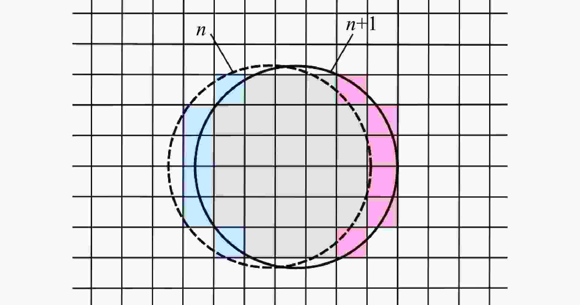
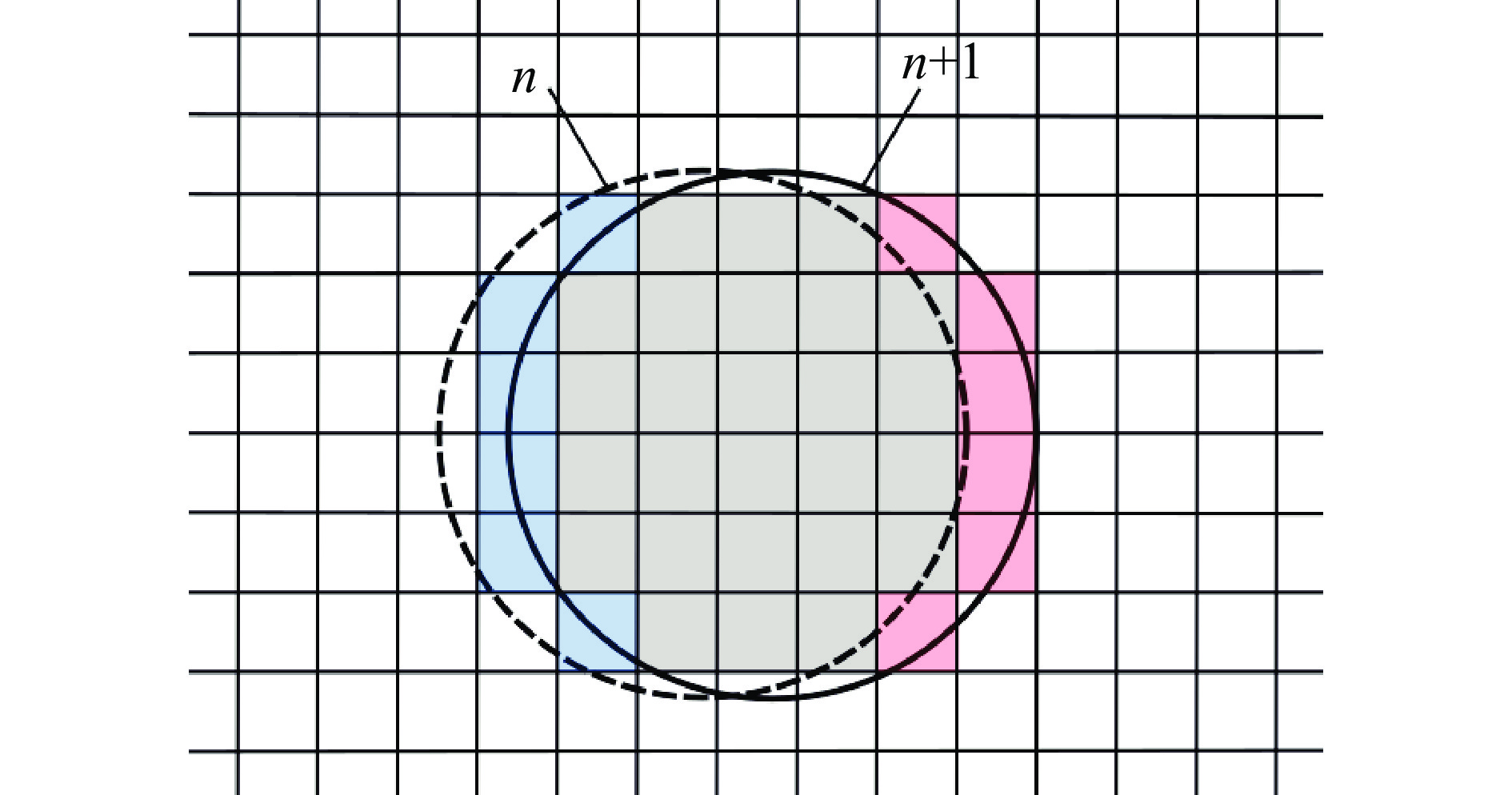
图 2 从 ${t_n}$ 时刻到 ${t_{n + 1}}$ 时刻边界进行移动，造成红色的失效单元和蓝色的新增单元

Figure 2. Boundary motion on a fixed grid from time ${t_n}$ to ${t_{n + 1}}$ . Dead (red) and fresh (blue) cells are generated by the motion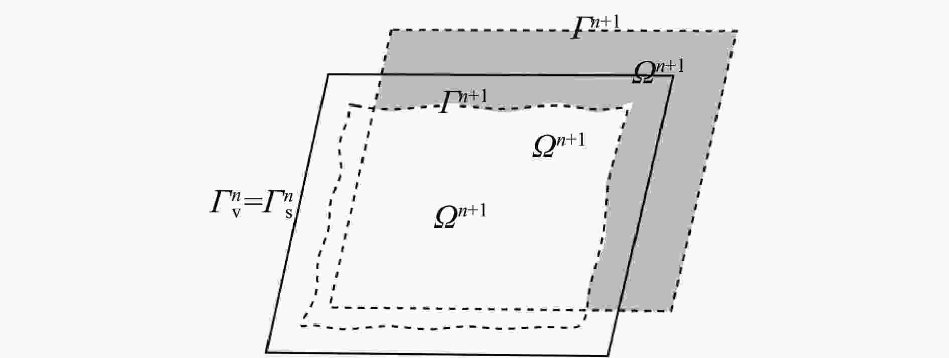

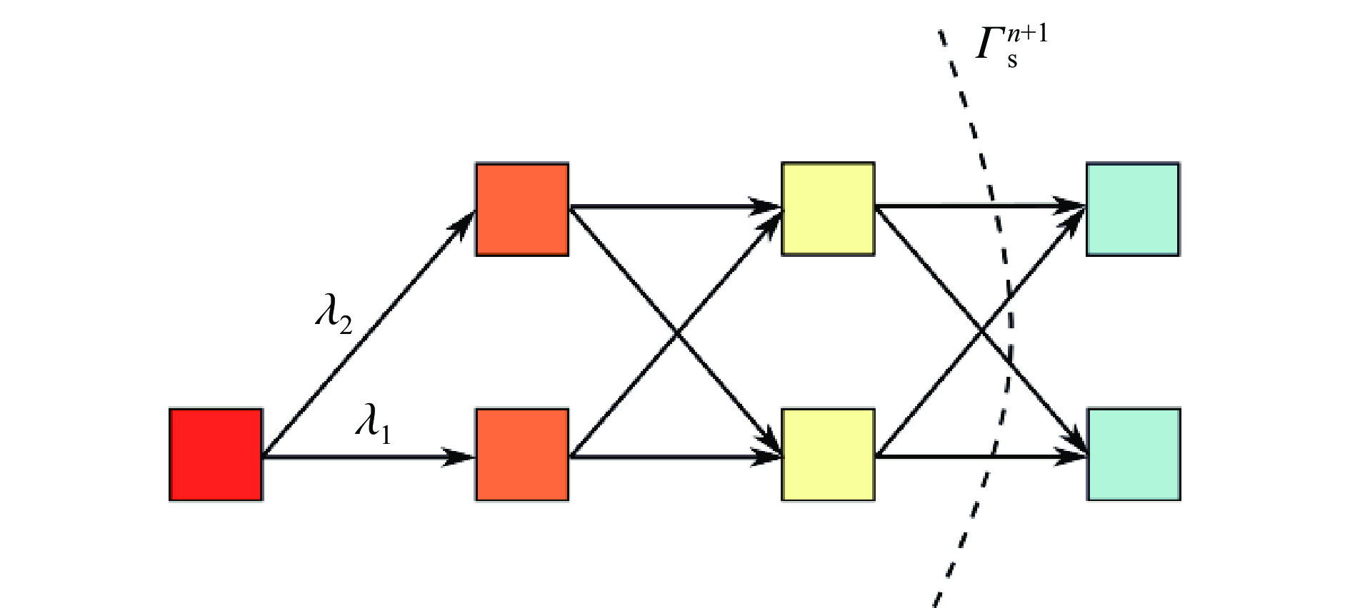
下载: 全尺寸图片幻灯片

图 3 流固耦合系统的子域变化（实线代表 ${t_n}$ 时刻的边界，虚线代表 ${t_{n + 1}}$ 时刻的边界）

Figure 3. Changes of the subdomains of the fluid-structure interaction system, where solid lines are boundaries at ${t_n}$ , and dashed lines are boundaries at ${t_{n + 1}}$

下载: 全尺寸图片幻灯片

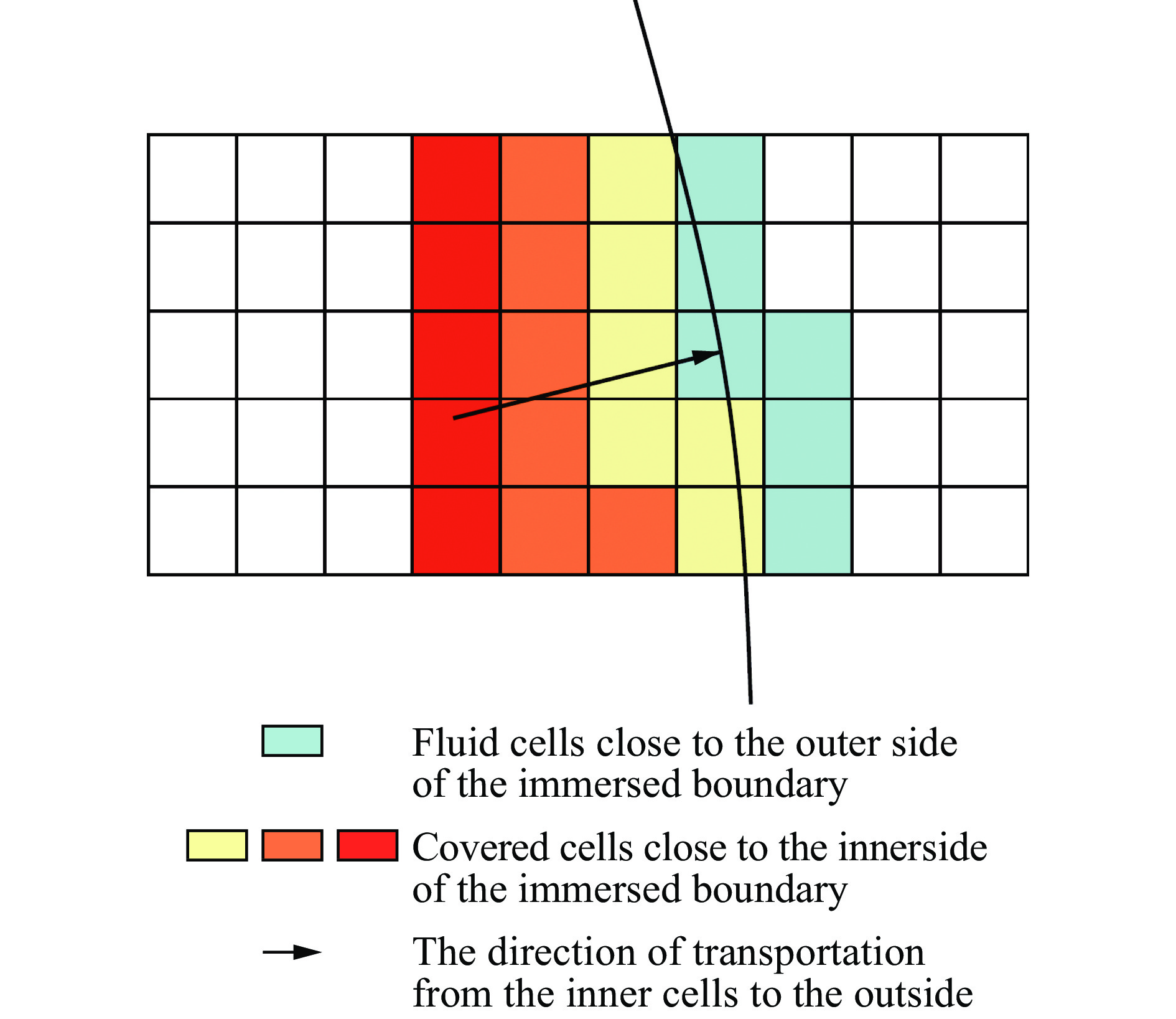
图 4 流体标记和输运方向，曲线为浸入边界

Figure 4. Fluid markers and direction of transportation, the curve is the immersed boundary

下载: 全尺寸图片幻灯片

图 5 依据染色顺序逐层输运流体

Figure 5. Transport the fluid in sequence of colors

下载: 全尺寸图片幻灯片

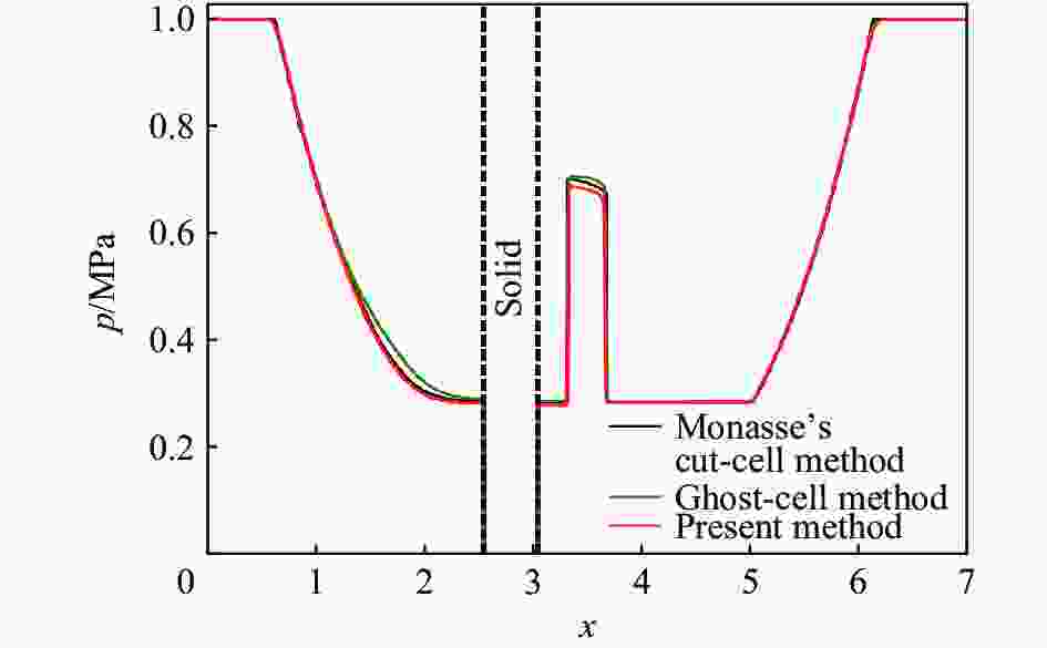
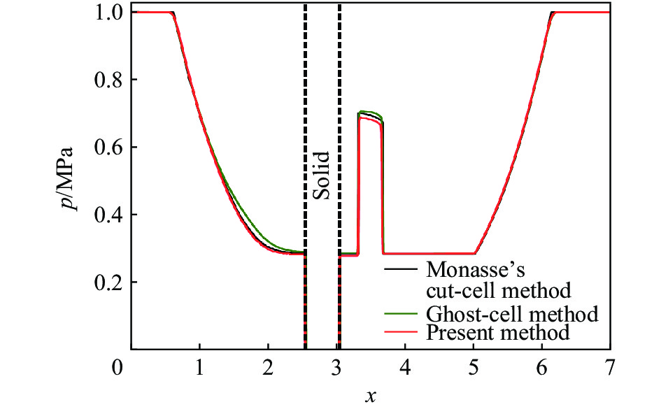
图 6 t=0.003时刻的压力分布（网格数为1 440，虚线表示浸入边界）

Figure 6. Pressure distribution at t=0.003 (The number of cells is1 440, and the dashed lines stand for the immersed boundaries.)

下载: 全尺寸图片幻灯片

图 7 流体相对质量的历史曲线

Figure 7. History of the relative mass of the fluid

下载: 全尺寸图片幻灯片

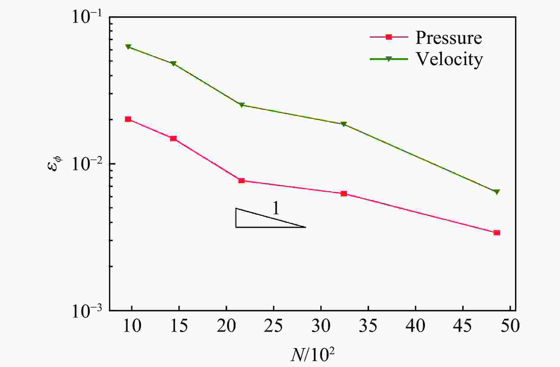
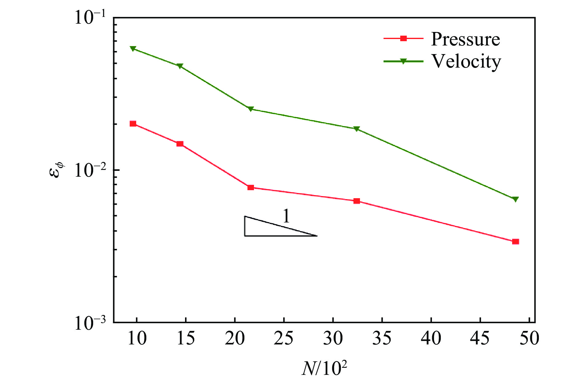
图 8 压力和速度的无量纲L2范数误差

Figure 8. Dimensionless L2 norms of error of the pressure and velocity

下载: 全尺寸图片幻灯片

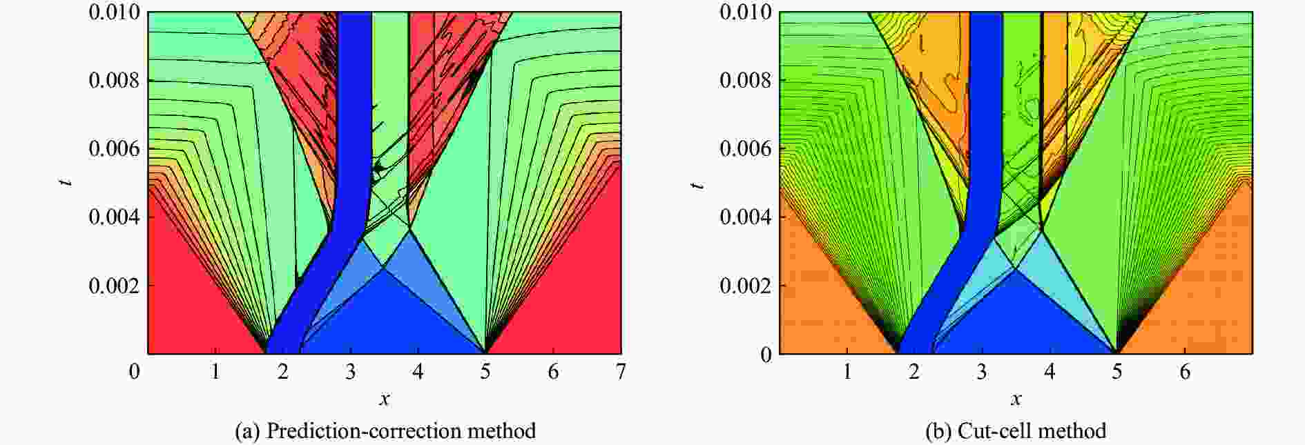
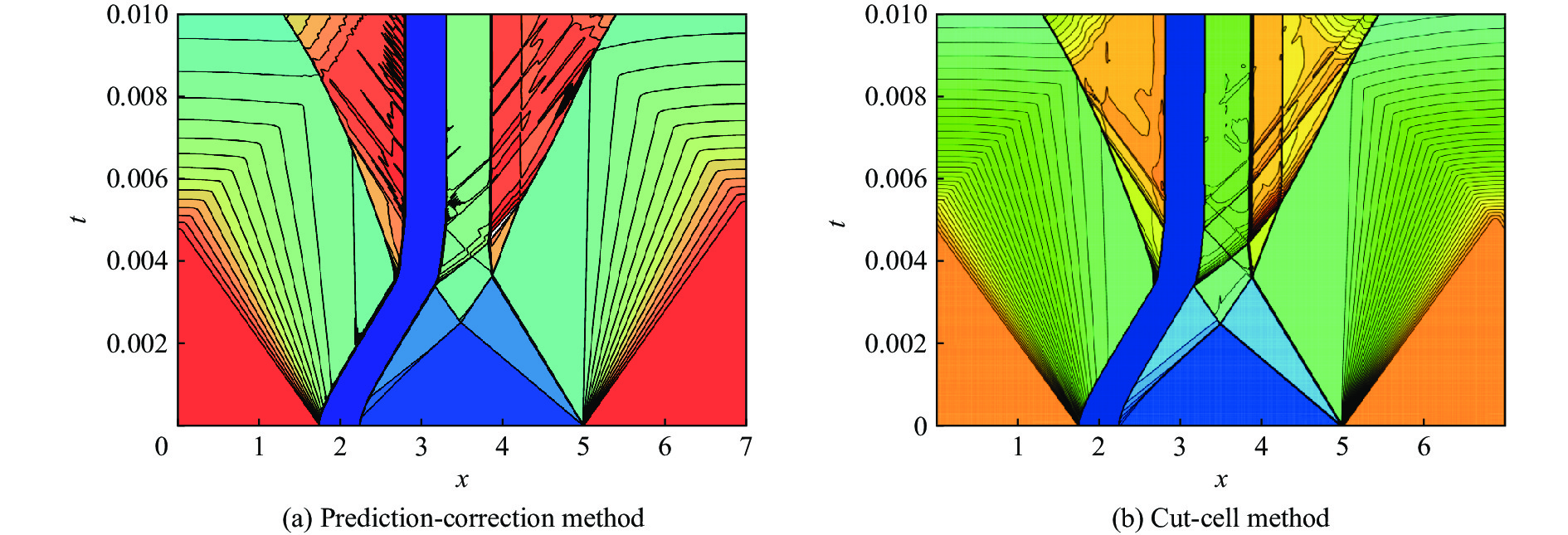
图 9 两种方法获得的流场密度 $\rho (x,t)$ 云图

Figure 9. Mass density $\rho (x,t)$ contours of the fluid by two methods

下载: 全尺寸图片幻灯片

图 10 激波管初始条件（蓝色部分为有机玻璃板，灰色部分为静止流场，右侧红色部分为输入边界）

Figure 10. Initial conditions of the shock tube (The PMMA panel is blue, the static fluid is grey, the right boundary in red color is the inflow.)

下载: 全尺寸图片幻灯片

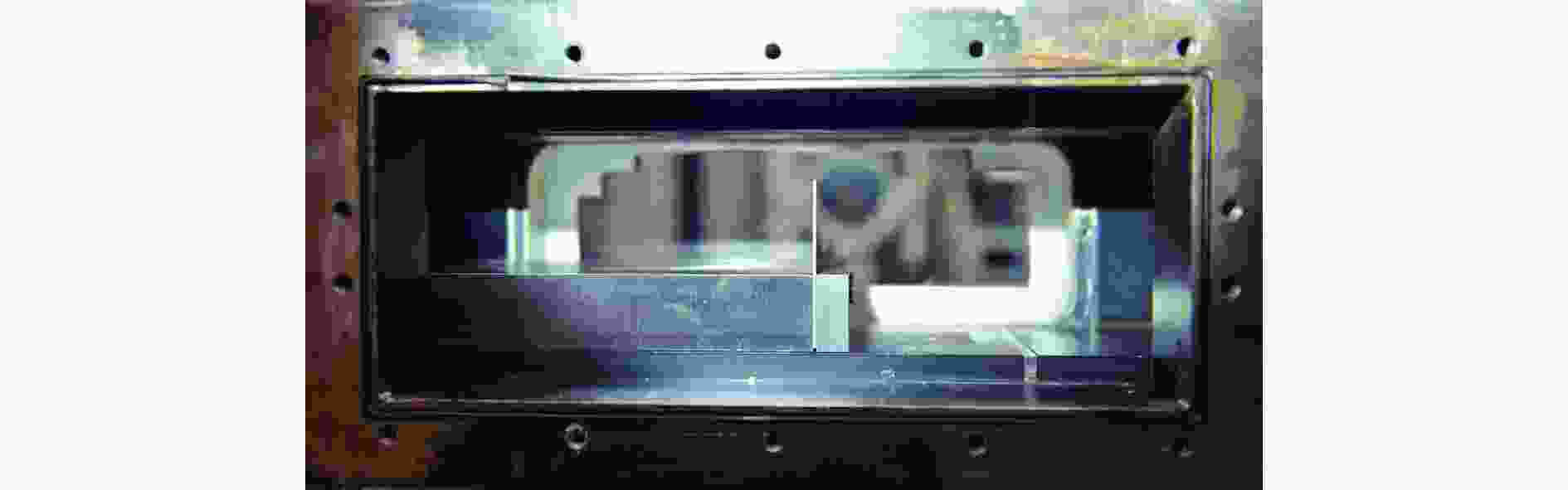
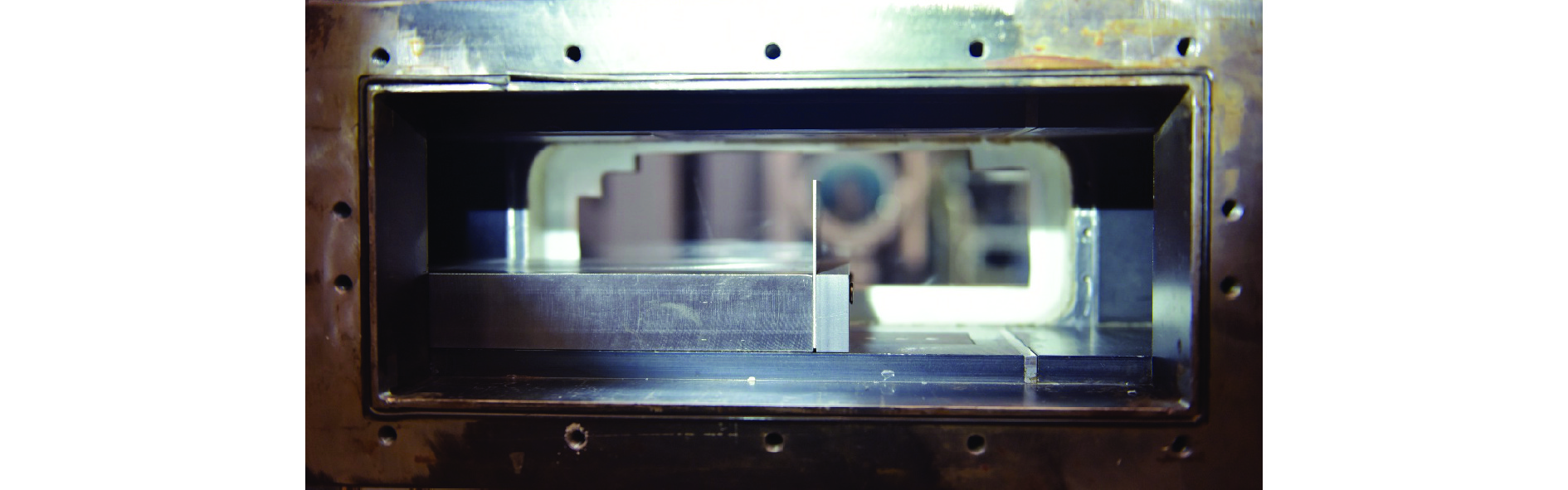
图 11 激波管实验段（底部的金属方块为基座，竖立薄片为实验测量的平板）

Figure 11. Experimental section of the shock tube (The metal block on the bottom is the base, and the vertical sheet is the tested panel.)

下载: 全尺寸图片幻灯片

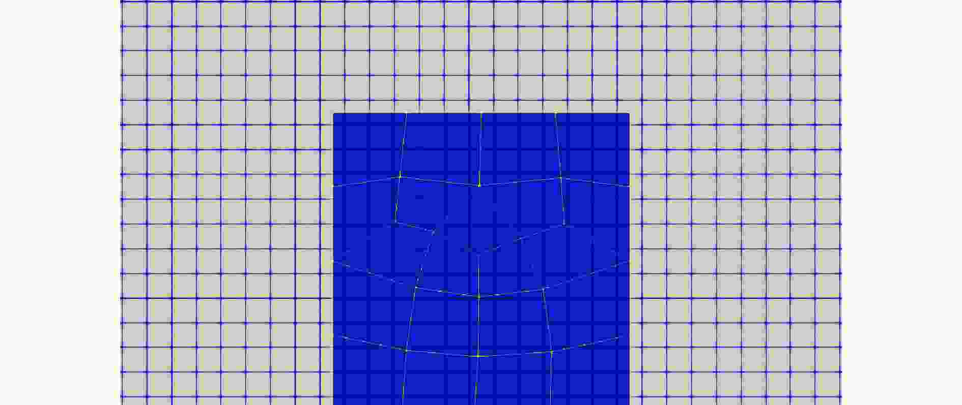
图 12 局部网格（灰色部分为流场，蓝色部分为平板）

Figure 12. Local grids (The fluid is grey, and the panel is blue.)

下载: 全尺寸图片幻灯片

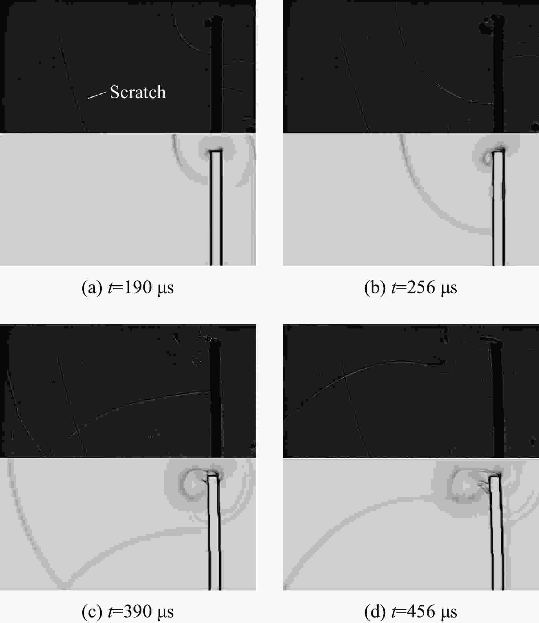
图 13 不同时刻实验纹影与模拟纹影的对比

Figure 13. Comparison of experimental and simulated shadowgraphs

下载: 全尺寸图片幻灯片

图 14 平板的最大挠度

Figure 14. Maximum deflections of the panel

下载: 全尺寸图片幻灯片

参考文献(39)

[1]	PESKIN C S. Flow patterns around heart valves: a numerical method [J]. Journal of Computational Physics, 1972, 10(2): 252–271. DOI: 10.1016/0021-9991(72)90065-4.
[2]	PESKIN C S. Numerical analysis of blood flow in the heart [J]. Journal of Computational Physics, 1977, 25(3): 220–252. DOI: 10.1016/0021-9991(77)90100-0.
[3]	王力, 田方宝. 浸入边界法及其在可压缩流动中的应用和进展 [J]. 中国科学: 物理学力学天文学, 2018, 48(9): 094703. DOI: 10.1360/SSPMA2018-00191. WANG L, TIAN F B. Recent progress of immersed boundary method and its applications in compressible fluid flow [J]. Scientia Sinica Physica, Mechanica & Astronomica, 2018, 48(9): 094703. DOI: 10.1360/SSPMA2018-00191.
[4]	SEO J H, MITTAL R. A high-order immersed boundary method for acoustic wave scattering and low-Mach number flow-induced sound in complex geometries [J]. Journal of Computational Physics, 2011, 230(4): 1000–1019. DOI: 10.1016/j.jcp.2010.10.017.
[5]	王力, 田方宝. 弹性拍翼悬停时的流固耦合效应 [J]. 气体物理, 2020, 5(4): 21–30. DOI: 10.19527/j.cnki.2096-1642.0812. WANG L, TIAN F B. Fluid-structure interaction of flexible flapping wing in hovering flight [J]. Physics of Gases, 2020, 5(4): 21–30. DOI: 10.19527/j.cnki.2096-1642.0812.
[6]	CHENG L, DU L, WANG X Y, et al. A semi-implicit immersed boundary method for simulating viscous flow-induced sound with moving boundaries [J]. Computer Methods in Applied Mechanics and Engineering, 2021, 373: 113438. DOI: 10.1016/j.cma.2020.113438.
[7]	赵西增, 付英男, 张大可, 等. 紧致插值曲线方法在流向强迫振荡圆柱绕流中的应用 [J]. 力学学报, 2015, 47(3): 441–450. DOI: 10.6052/0459-1879-14-387. ZHAO X Z, FU Y N, ZHANG D K, et al. Application of a CIP-based numerical simulation of flow past an in-line forced oscillating circular cylinder [J]. Chinese Journal of Theoretical and Applied Mechanics, 2015, 47(3): 441–450. DOI: 10.6052/0459-1879-14-387.
[8]	段松长, 赵西增, 叶洲腾, 等. 错列角度对双圆柱涡激振动影响的数值模拟研究 [J]. 力学学报, 2018, 50(2): 244–253. DOI: 10.6052/0459-1879-17-345. DUAN S C, ZHAO X Z, YE Z T, et al. Numerical study of staggered angle on the vortex-induced vibration of two cylinders [J]. Chinese Journal of Theoretical and Applied Mechanics, 2018, 50(2): 244–253. DOI: 10.6052/0459-1879-17-345.
[9]	杨明, 刘巨保, 岳欠杯, 等. 涡激诱导并列双圆柱碰撞数值模拟研究 [J]. 力学学报, 2019, 51(6): 1785–1796. DOI: 10.6052/0459-1879-19-224. YANG M, LIU J B, YUE Q B, et al. Numerical simulation on the vortex-induced collision of two side-by-side cylinders [J]. Chinese Journal of Theoretical and Applied Mechanics, 2019, 51(6): 1785–1796. DOI: 10.6052/0459-1879-19-224.
[10]	陈威霖, 及春宁, 许栋. 不同控制角下附加圆柱对圆柱涡激振动影响 [J]. 力学学报, 2019, 51(2): 432–440. DOI: 10.6052/0459-1879-18-208. CHEN W L, JI C N, XU D. Effects of the added cylinders with different control angles on the vortex-induced vibrations of a circular cylinder [J]. Chinese Journal of Theoretical and Applied Mechanics, 2019, 51(2): 432–440. DOI: 10.6052/0459-1879-18-208.
[11]	HOSSEINJANI A A, ROOHI A H. Immersed boundary method for MHD unsteady natural convection around a hot elliptical cylinder in a cold rhombus enclosure filled with a nanofluid [J]. SN Applied Sciences, 2021, 3(2): 270. DOI: 10.1007/s42452-021-04221-3.
[12]	YE H X, CHEN Y, MAKI K. A discrete-forcing immersed boundary method for turbulent-flow simulations [J]. Proceedings of the Institution of Mechanical Engineers, 2021, 235(1): 188–202. DOI: 10.1177/1475090220927245.
[13]	SOTIROPOULOS F, YANG X. Immersed boundary methods for simulating fluid-structure interaction [J]. Progress in Aerospace Sciences, 2014, 65: 1–21. DOI: 10.1016/j.paerosci.2013.09.003.
[14]	YOUSEFZADEH M, BATTIATO I. High order ghost-cell immersed boundary method for generalized boundary conditions [J]. International Journal of Heat and Mass Transfer, 2019, 137: 585–598. DOI: 10.1016/j.ijheatmasstransfer.2019.03.061.
[15]	吴晓笛, 刘华坪, 陈浮. 基于浸入边界-多松弛时间格子玻尔兹曼通量求解法的流固耦合算法研究 [J]. 物理学报, 2017, 66(22): 224702. DOI: 10.7498/aps.66.224702. WU X D, LIU H P, CHEN F. A method combined immersed boundary with multi-relaxation-time lattice Boltzmann flux solver for fluid-structure interaction [J]. Acta Physica Sinica, 2017, 66(22): 224702. DOI: 10.7498/aps.66.224702.
[16]	BOUKHARFANE R, EUGȆNIO RIBEIRO F H, BOUALI Z, et al. A combined ghost-point-forcing/direct-forcing immersed boundary method (IBM) for compressible flow simulations [J]. Computers and Fluids, 2018, 162: 91–112. DOI: 10.1016/j.compfluid.2017.11.018.
[17]	MAJUMDAR S, IACCARINO G, DURBIN P. RANS solvers with adaptive structured boundary non-conforming grids [J]. Center for Turbulence Research. Annual Research Briefs, 2001: 353–366.
[18]	朱祥德, 陈春刚, 肖锋. 一种基于多矩的有限体积浸入边界法 [J]. 计算物理, 2010, 27(3): 342–352. DOI: 10.19596/j.cnki.1001-246x.2010.03.004. ZHU X D, CHEN C G, XIAO F. A multi-moment immersed-boundary finite-volume scheme [J]. Chinese Journal of Computational Physics, 2010, 27(3): 342–352. DOI: 10.19596/j.cnki.1001-246x.2010.03.004.
[19]	LEE J M, YOU D H. An implicit ghost-cell immersed boundary method for simulations of moving body problems with control of spurious force oscillations [J]. Journal of Computational Physics, 2013, 233(1): 295–314. DOI: 10.1016/j.jcp.2012.08.044.
[20]	辛建建, 石伏龙, 金秋. 一种径向基函数虚拟网格法数值模拟复杂边界流动 [J]. 物理学报, 2017, 66(4): 044704. DOI: 10.7498/aps.66.044704. XIN J J, SHI F L, JIN Q. Numerical simulation of complex immersed boundary flow by a radial basis function ghost cell method [J]. Acta Physica Sinica, 2017, 66(4): 044704. DOI: 10.7498/aps.66.044704.
[21]	XIN J J, LI T Q, SHI F L. A radial basis function for reconstructing complex immersed boundaries in ghost cell method [J]. Journal of Hydrodynamics, 2018, 30(5): 890–897. DOI: 10.1007/s42241-018-0097-3.
[22]	石伏龙, 辛建建, 马麟. 梯度增量level set/虚拟网格法模拟波浪结构物相互作用 [J]. 工程热物理学报, 2018, 39(11): 2420–2428. SHI F L, XIN J J, MA L. A gradient-augmented level set/ghost cell method for the simulation of wave structure interaction [J]. Journal of Engineering Thermophysics, 2018, 39(11): 2420–2428.
[23]	QU Y G, SHI R C, BATRA R C. An immersed boundary formulation for simulating high-speed compressible viscous flows with moving solids [J]. Journal of Computational Physics, 2018, 354: 672–691. DOI: 10.1016/j.jcp.2017.10.045.
[24]	HAJI MOHAMMADI M, SOTIROPOULOS F, BRINKERHOFF J. Moving least squares reconstruction for sharp interface immersed boundary methods [J]. International Journal for Numerical Methods, 2019, 90(2): 57–80. DOI: 10.1002/fld.4711.
[25]	雷悦, 石伏龙. 虚拟网格法模拟静止或运动并列布置双圆柱绕流现象 [J]. 工程热物理学报, 2020, 41(8): 1974–1983. LEI Y, SHI F L. A ghost cell method for simulating flows around stationary of moving twin cylinders in a side-by-side arrangement [J]. Journal of Engineering Thermophysics, 2020, 41(8): 1974–1983.
[26]	XIE F T, QU Y G, ISLAM M A, et al. A sharp-interface Cartesian grid method for time-domain acoustic scattering from complex geometries [J]. Computers and Fluids, 2020, 202: 104498. DOI: 10.1016/j.compfluid.2020.104498.
[27]	CHI C, ABDELSAMIE A, THÉVENIN D. A directional ghost-cell immersed boundary method for incompressible flows [J]. Journal of Computational Physics, 2020, 404: 109122. DOI: 10.1016/j.jcp.2019.109122.
[28]	ZHENG K Y, ZHAO X Z, YANG Z J, et al. Numerical simulation of water entry of a wedge using a modified ghost-cell immersed boundary method [J]. Journal of Marine Science and Technology, 2020, 25(2): 589–608. DOI: 10.1007/s00773-019-00666-9.
[29]	CLARKE D K, HASSAN H A, SALAS M D. Euler calculations for multielement airfoils using Cartesian grids [J]. AIAA Journal, 1986, 24(3): 353–358. DOI: 10.2514/3.9273.
[30]	MEYER M, DEVESA A, HICKEL S, et al. A conservative immersed interface method for large-eddy simulation of incompressible flows [J]. Journal of Computational Physics, 2010, 229(18): 6300–6317. DOI: 10.1016/j.jcp.2010.04.040.
[31]	MONASSE L, DARU V, MARIOTTI C, et al. A conservative coupling algorithm between a compressible flow and a rigid body using an embedded boundary method [J]. Journal of Computational Physics, 2012, 231(7): 2977–2994. DOI: 10.1016/j.jcp.2012.01.002.
[32]	SCHNEIDERS L, GÜNTHER C, MEINKE M, et al. An efficient conservative cut-cell method for rigid bodies interacting with viscous compressible flows [J]. Journal of Computational Physics, 2016, 311: 62–86. DOI: 10.1016/j.jcp.2016.01.026.
[33]	BRADY P T, LIVESCU D. Foundations for high-order, conservative cut-cell methods: stable discretizations on degenerate meshes [J]. Journal of Computational Physics, 2021, 426: 109794. DOI: 10.1016/j.jcp.2020.109794.
[34]	SEO J H, MITTAL R. A sharp-interface immersed boundary method with improved mass conservation and reduced spurious pressure oscillations [J]. Journal of Computational Physics, 2011, 230(19): 7347–7363. DOI: 10.1016/j.jcp.2011.06.003.
[35]	张德良. 计算流体力学教程[M]. 北京: 高等教育出版社, 2010: 279–288. ZHANG D L. A course in computational fluid dynamics [M]. Beijing: Higher Education Press, 2010: 279–288.
[36]	TORO E F, VÁZQUEZ-CENDÓN M E. Flux splitting schemes for the Euler equations [J]. Computers and Fluids, 2012, 70: 1–12. DOI: 10.1016/j.compfluid.2012.08.023.
[37]	LIOU M S. A sequel to AUSM, part II: AUSM⁺-up for all speeds [J]. Journal of Computational Physics, 2006, 214(1): 137–170. DOI: 10.1016/j.jcp.2005.09.020.
[38]	王勖成. 有限单元法[M]. 北京: 清华大学出版社, 2003. WANG X C. Finite element method [M]. Beijing: Tsinghua University Press, 2003.
[39]	李亭鹤, 阎超. 一种新的分区重叠洞点搜索方法-感染免疫法 [J]. 空气动力学学报, 2001, 19(2): 156–160. DOI: 10.3969/j.issn.0258-1825.2001.02.004. LI T H, YAN C. A new method of hole-point search in grid embedding technique [J]. Acta Aerodynamica Sinica, 2001, 19(2): 156–160. DOI: 10.3969/j.issn.0258-1825.2001.02.004.