


SPH-HLLC coupled method for one-dimentional elastic-perfectly plastic model
-
摘要: 通过弹塑性波分析求得HLLC(Harten-Lax-van Leer-contact)近似黎曼解,提出了SPH(smoothed particle hydrodynamics)与一维理想弹塑性体模型下近似的HLLC黎曼求解器耦合的一种构造简单的算法。在SPH计算中,支持域内每个粒子对都存在一个黎曼间断问题,它的黎曼解被代入控制方程中计算。其中一维理想弹塑性体的HLLC近似黎曼解的思想是:先假设整体处于弹性状态计算黎曼解,然后对计算结果进行塑性条件修正,最后用修正后的物理变量计算HLLC近似黎曼解。将提出的SPH-HLLC耦合算法与传统SPH算法在一维算例下的计算结果进行对比,结果表明,该算法能有效模拟一维理想弹塑性体材料的碰撞,并能有效抑制在不同材料之间的压强和偏应力震荡,这是传统SPH方法很难做到的。Abstract: A 1D SPH (smoothed particle hydrodynamics) and approximate HLLC (Harten-Lax-van Leer-contact) Riemann solver coupled method for elastic-perfectly plastic model is proposed through elastic and plastic wave analysis. In SPH simulations, each particle pair in the supporting domain generates a Riemann problem, whose solutions are substituted into governing equations. The philosophy of HLLC approximate Riemann solver is to divide the procedure into three steps: assume the whole state in elastic deformation and compute Riemann problem, and then reconstruct flux under von Mises yielding conditions and compute the final HLLC Riemann solution with reconstructed fluxes. We compare the new SPH-HLLC method with the traditional SPH method in several numerical tests, which show that this method can effectively simulate collision and reflected rarefaction waves between the materials, and it can profoundly suppress oscillations of pressure and deviatoric stress at contact interface between different materials, which the traditional SPH method finds difficult to realize. Moreover, the new SPH-HLLC scheme shows better energy performance than the traditional SPH method in 2D test case where initial kinetic energy is successfully transformed into internal energy with new SPH-HLLC scheme while total energy significantly decreases with time using the traditional SPH method.
-

图 1 铝碰撞算例的密度、压强、速度和偏应力计算结果
Figure 1. Density, pressure, velocity and deviatoric stress profile of Al collision test

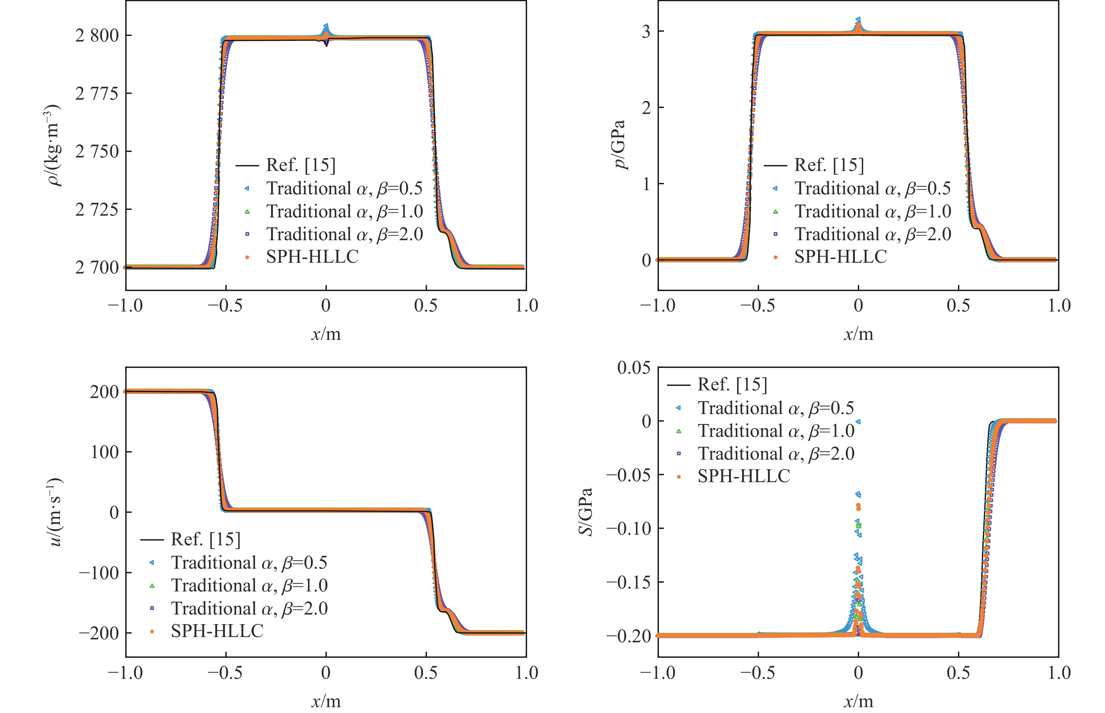
图 2 Wilkins算例的密度、压强、速度和偏应力计算结果
Figure 2. Density, pressure, velocity and deviatoric stress profile of Wilkins test

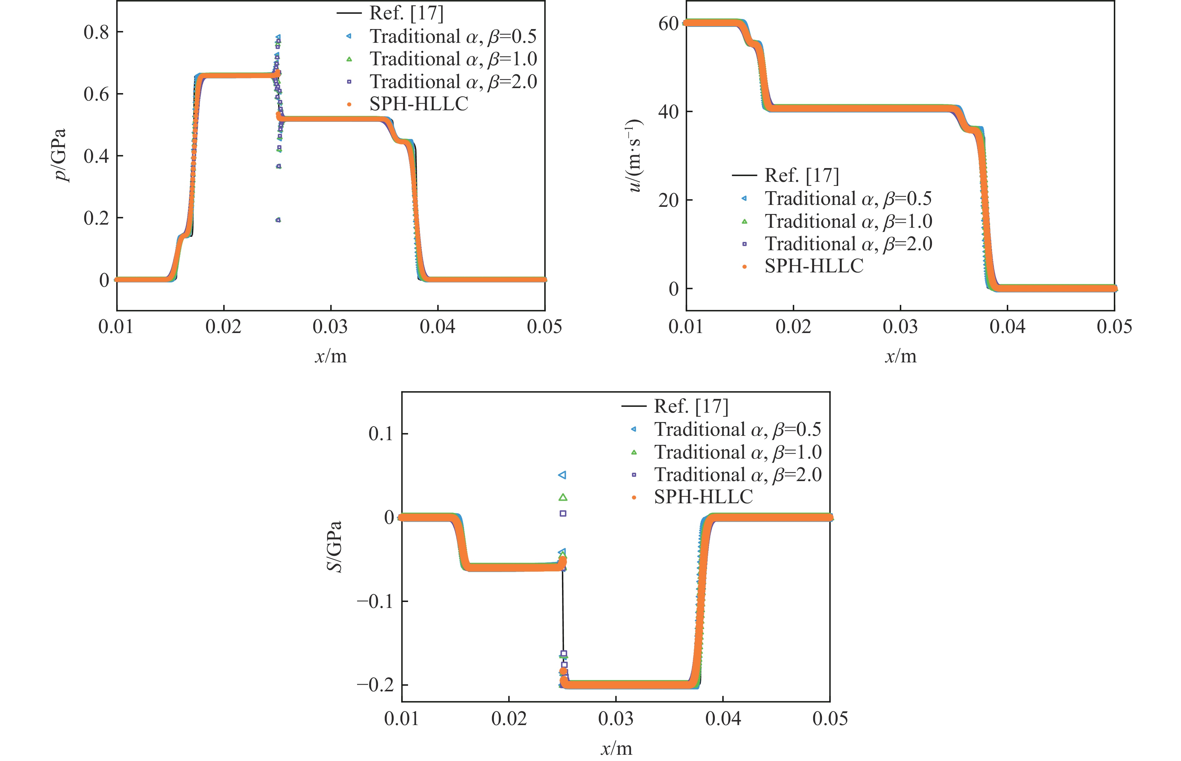
图 3 铜铝撞击算例的压强、速度和偏应力计算结果
Figure 3. Pressure, velocity and deviatoric stress profile of Cu/Al collision test

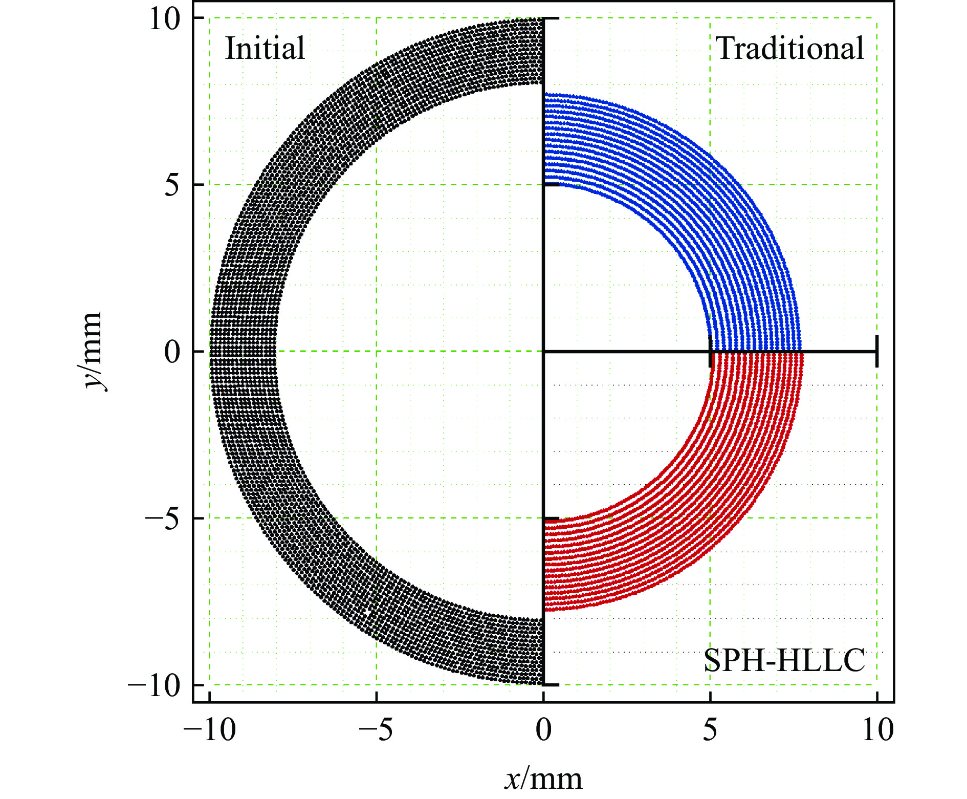
图 4 二维厚壁圆筒铍壳体碰撞测试的初始分布、传统算法结果以及新SPH-HLLC算法结果
Figure 4. Initial distribution, traditional algorithm results, and new SPH-HLLC algorithm results of two-dimensional thick walled cylindrical beryllium shell collision test

图 5 二维厚壁圆筒铍壳体碰撞测试的无量纲能量随无量纲时间的变化
Figure 5. Variation of non-dimensional energy with non-dimensional time in collision test of two-dimensional thick walled cylindrical beryllium shells
表 1 弹塑性碰撞测试
Table 1. Parameters related Al impact
算例 ρ/(kg·m−3) u/(m·s−1) p/MPa S/MPa 坐标区间/m t/ms 铝碰撞 左侧 2700 200 0 −200 −1~0 0.1 右侧 2700 −200 0 0 0~1  下载: 导出CSV
表 2 Wilkins算例的相关参数
Table 2. Parameters related to Wilkins test
算例 ρ/(kg·m−3) u/(m·s−1) Y0/MPa μ/GPa a0/(m·s−1) ρ0/(kg·m−3) s Γ0 坐标区间/mm t/μs Wilkins 左侧 2785 800 300 27.6 5328 2785 1.338 2 0 ~ 5 5 右侧 2785 0 300 27.6 5328 2785 1.338 2 5 ~ 50
下载: 导出CSV
表 3 铜铝材料撞击算例的相关参数
Table 3. Parameters related to Cu/Al collision
算例 ρ/(kg·m−3) u/(m·s−1) Y0/MPa μ/GPa a0/(m·s−1) ρ0/(kg·m−3) s Γ0 坐标区间/mm t/μs 铜铝材料撞击 左侧 8930 60 90 45.0 3940 8930 1.490 2 0 ~ 25 2 右侧 2785 0 300 27.6 5328 2785 1.338 2 25~50
下载: 导出CSV
表 4 二维厚壁圆筒铍壳体碰撞算例的相关参数
Table 4. Parameters related to collapse of a thick-walled cylindrical beryllium shell
算例 ρ0/(kg·m−3) |u|/(m·s−1) Y0/MPa μ/GPa a0/(m·s−1) s Γ t/μs 铍壳体 1845 417.1 330 151.9 12870 1.124 2 130
下载: 导出CSV
表 5 计算前后总能比(结束时刻能量/初始时刻能量)
Table 5. Total energy ratio (final total energy/initial total energy)
方法 总能比/% l0 = 0.2 mm l0 = 0.125 mm l0 = 0.08 mm 传统 90.40 92.75 94.69 SPH-HLLC 100.59 100.72 100.64
下载: 导出CSV
-
[1] MONAGHAN J J. Smoothed particle hydrodynamics [J]. Annual Review of Astronomy and Astrophysics, 1992, 30: 543–574. DOI: 10.1146/annurev.aa.30.090192.002551. [2] VILA J P. On particle weighted methods and smooth particle hydrodynamics [J]. Mathematical Models and Methods in Applied Sciences, 1999, 9(2): 161–209. DOI: 10.1142/S0218202599000117. [3] PARSHIKOV A N, MEDIN S A. Smoothed particle hydrodynamics usinginterparticle contact algorithms [J]. Journal of Computational Physics, 2002, 180(1): 358–382. DOI: 10.1006/jcph.2002.7099. [4] LIBERSKY L D, RANDLES P W. Shocks and discontinuities in particle methods [J]. AIP Conference Proceedings, 2006, 845(1): 1089–1092. DOI: 10.1063/1.2263512. [5] MEHRA V, CHATURVEDI S. High velocity impact of metal sphere on thin metallic plates: a comparative smooth particle hydrodynamics study [J]. Journal of Computational Physics, 2006, 212(1): 318–337. DOI: 10.1016/j.jcp.2005.06.020. [6] LIN X, BALLMANN J. A Riemann solver and a second-order Godunov method for elastic-plastic wave propagation in solids [J]. International Journal of Impact Engineering, 1993, 13(3): 463–478. DOI: 10.1016/0734-743X(93)90118-Q. [7] 姚成宝, 付梅艳, 韩峰, 等. 基于多介质Riemann问题的流体-固体耦合数值方法及其在爆炸与冲击问题中的应用 [J]. 兵工学报, 2021, 42(2): 340–355. DOI: 10.3969/j.issn.1000-1093.2021.02.012.YAO C B, FU M Y, HAN F, et al. A numerical scheme for fluid-solid interactions based on multi-medium Riemann problem and its application in explosion andimpact problems [J]. Acta Armamentarii, 2021, 42(2): 340–355. DOI: 10.3969/j.issn.1000-1093.2021.02.012. [8] CHENG J B. Harten-Lax-van Leer-contact (HLLC) approximation Riemann solver with elastic waves for one-dimensional elastic-plastic problems [J]. Applied Mathematics and Mechanics, 2016, 37(11): 1517–1538. DOI: 10.1007/s10483-016-2104-9. [9] GAO S, LIU T G. 1D exact elastic-perfectly plastic solid Riemann solver and its multi-material application [J]. Advances in Applied Mathematics and Mechanics, 2017, 9(3): 621–650. DOI: 10.4208/aamm.2015.m1340. [10] GAO S, LIU T G, YAO C B. A complete list of exact solutions for one-dimensional elastic-perfectly plastic solid Riemann problem without vacuum [J]. Communications in Nonlinear Science and Numerical Simulation, 2018, 63: 205–227. DOI: 10.1016/j.cnsns.2018.02.030. [11] LI X, ZHAI J Y, SHEN Z J. An HLLC-type approximate Riemann solver for two-dimensional elastic-perfectly plastic model [J]. Journal of Computational Physics, 2022, 448: 110675. DOI: 10.1016/j.jcp.2021.110675. [12] LIU M B, LIU G R. Smoothed particle hydrodynamics (SPH): an overview and recent developments [J]. Archives of Computational Methods in Engineering, 2010, 17(1): 25–76. DOI: 10.1007/s11831-010-9040-7. [13] HUI W H, KUDRIAKOV S. On wall overheating and other computational difficulties of shock-capturing methods [J]. Computational Fluid Dynamics Journal, 2001, 10(2): 192–209. [14] TORO E F. Riemann solvers and numerical methods for fluid dynamics: a practical introduction [M]. New York: Springer, 1997. [15] CHEN Q, LI L, QI J, et al. A cell-centeredLagrangian scheme with an elastic-perfectly plastic solid Riemann solver for wave propagations in solids [J]. Advances in Applied Mathematics and Mechanics, 2022, 14(3): 703–724. DOI: 10.4208/aamm.OA-2020-0344. [16] WILKINS M L. Calculation of elastic-plastic flow: NSA-18-002406 [R]. Livermore: Lawrence Radiation Laboratory, 1963. [17] LIU L, CHENG J B, LIU Z. A multi-material HLLC Riemann solver with both elastic and plastic waves for 1D elastic-plastic flows [J]. Computers & Fluids, 2019, 192: 104265. DOI: 10.1016/j.compfluid.2019.104265. [18] HOWELL B P, BALL G J. A free-Lagrange augmented Godunov method for the simulation of elastic-plastic solids [J]. Journal of Computational Physics, 2002, 175(1): 128–167. DOI: 10.1006/jcph.2001.6931. [19] MAIRE P H, ABGRALL R, BREIL J, et al. A nominally second-order cell-centered Lagrangian scheme for simulating elastic-plastic flows on two-dimensional unstructured grids [J]. Journal of Computational Physics, 2013, 235: 626–665. DOI: 10.1016/j.jcp.2012.10.017. [20] QUINLAN N J, BASA M, LASTIWKA M. Truncation error in mesh-free particle methods [J]. International Journal for Numerical Methods in Engineering, 2006, 66(13): 2064–2085. DOI: 10.1002/nme.1617. [21] ZHANG Z L, LIU M B. Smoothed particle hydrodynamics with kernel gradient correction for modeling high velocity impact in two- and three-dimensional spaces [J]. Engineering Analysis with Boundary Elements, 2017, 83: 141–157. DOI: 10.1016/j.enganabound.2017.07.015. -


计量
- 文章访问数: 487
- HTML全文浏览量: 154
- PDF下载量: 114
- 被引次数: 0